Worked examples
Download the project template (.zip) — the exact bundle to model yours on.
PHYS 3260
Download the project template (.zip) — the exact bundle to model yours on.
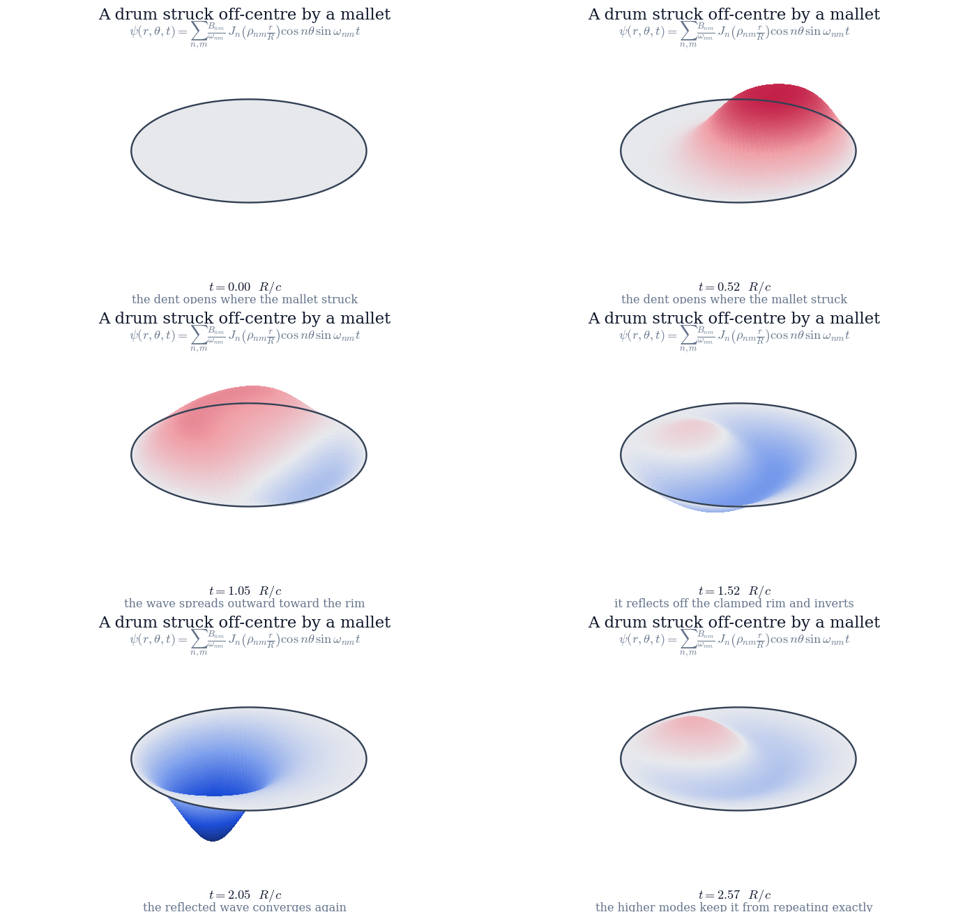 Why a Drum Has No Pitch: Modes of a Circular Membrane
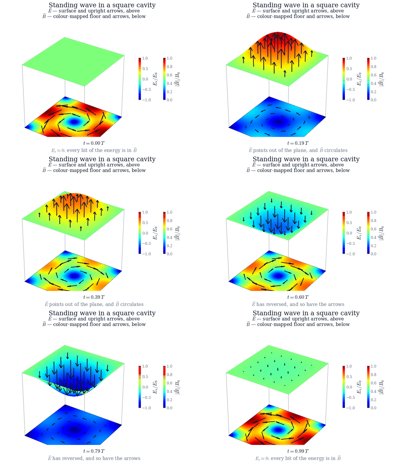 A Standing Electromagnetic Wave in a Square Cavity
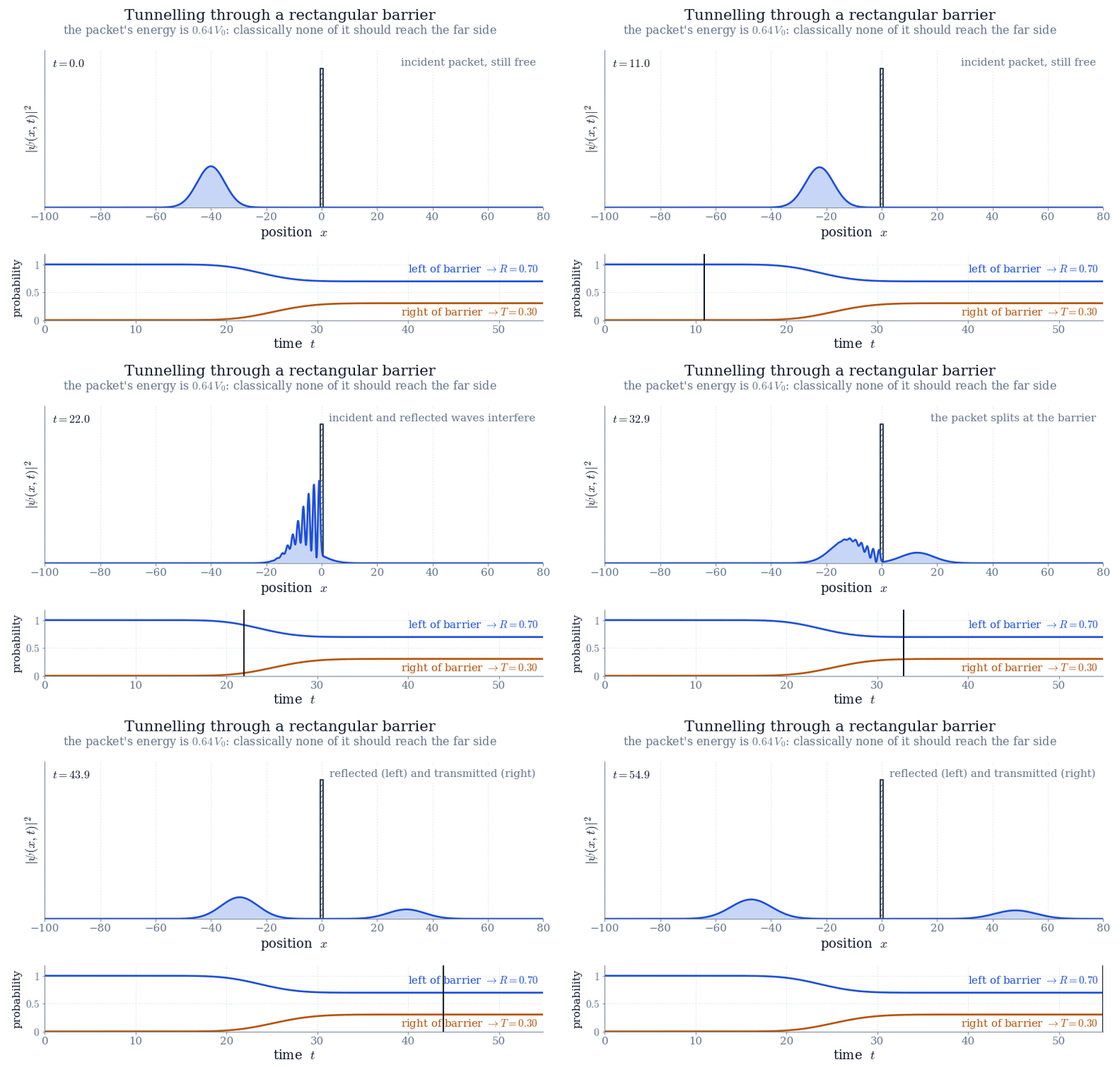 Quantum Tunnelling of a Wave Packet through a Rectangular Barrier (Numerical)
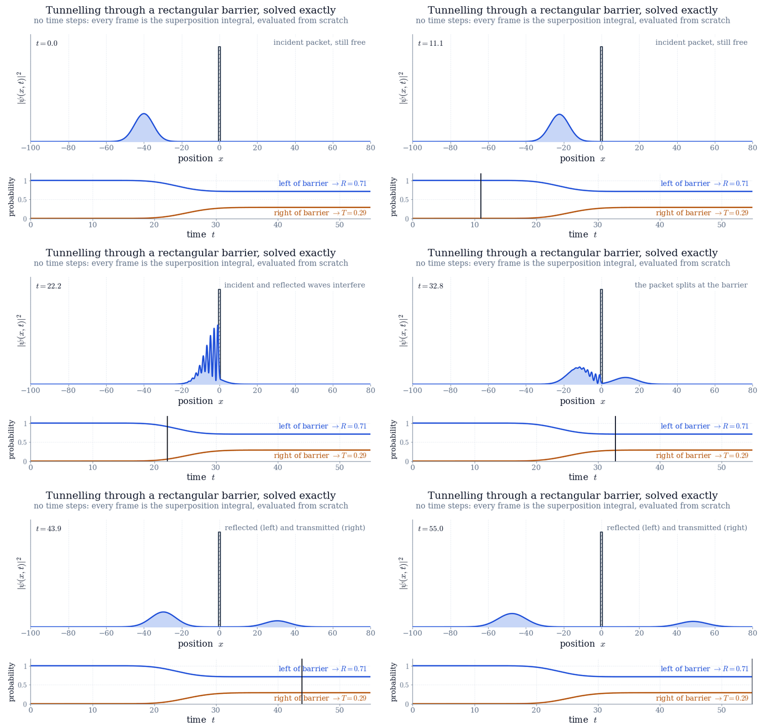 Quantum Tunnelling of a Wave Packet through a Rectangular Barrier (Analytical)
Pick a problem in physics or engineering that interests you. Solve it with the mathematical methods from this course, visualize the result, and write it up as a short report. The strongest reports are published on this page, where next year's students will read them.
The problem is yours to choose, but clear it with me before you start. Bring me one paragraph: what the question is, and which methods from this course will answer it. Something from your major, your research group or your job is ideal, because you already care how it comes out.
A proposal has to pass the same test the worked examples above pass: the mathematics of this course has to be doing the real work, not decorating a simulation. A useful way to check is to ask what is left if you take the computer away. If the answer is nothing — if the figures could have come out of a library routine without your ever writing down an equation — it is not a project for this course yet.
The project is worth 5% added on top of your course grade, so a perfect score in the rest of the course plus a good project comes to 105%. It is extra credit. Not doing it costs you nothing, and it is the cheapest 5% in the course.
You may use AI for any part of this. I would rather you did, and said so — it is how the work is done now. But that is exactly why the document you hand in cannot be the thing I grade: I cannot tell from a finished report who worked it out. So the grade comes from the ten-minute presentation. Expect to be asked, while you are standing there, why a particular step follows from the one above it, or what would change if some quantity in the problem were doubled. Those questions are hard to answer unless you have personally been through the derivation, and easy if you have. Build the project with whatever tools you like; be ready to defend every line of it.
Two things: the project folder and the presentation.
The project folder is a single .zip of one
folder named after your project. Inside it:
Maxwell/Maxwell.tex.figures/.Download the template above and build your folder out of it rather than from scratch. It is a complete project in exactly this layout, so anything you are unsure of is already answered there by example.
The ten-minute presentation — PowerPoint, Keynote or Beamer — covers the question, the mathematics, the figures and the conclusion, at roughly one slide per minute. Show the equations as they appear in your report; if your slide software sets mathematics badly, screenshot them from your PDF instead. Hand the presentation in on its own: it is not part of the project folder, and it is not published here.
Open with the problem. Directly under the title, before a
word of your own, put a problemstatement environment setting out
what is given and what is to be found, in lettered parts — the way every
worked example above opens. A reader needs to know what was asked before any of
the work below it means anything. Writing it first is also the cheapest way to
discover whether you have one problem or three. Your abstract goes immediately
under it, printed by \projectabstract, and everything from there
down is the report.
Name the methods where you use them. Write "separating the variables (Chapter 10)" or "the Fourier transform (Chapter 7)" at the line in the derivation where you actually do it, not only in a list at the end. Half the point of the project is recognizing this course inside a problem that was not written for it.
Make the animation the best thing you build. It is the preview that stands for your project on this page, and it is what decides whether anyone opens the project at all. Give it a caption that says what to watch for, so a reader knows what they are looking at before it loops.
Keep the code out of the report. The report is for the
physics and the mathematics. The code lives in code/, and the
figures are how the reader sees what it did.
Your .tex has to compile to a PDF on its own, and this website
renders that same file into the web page. So stay with ordinary LaTeX —
sections, equations, figures, lists — plus the four helper commands the
template defines. Do not rename them or change the order of their
arguments:
\projectinfo — your title, your name, and a one- or
two-sentence abstract. It prints the title and your name, and it is where
the heading of your card on this page comes from.\projectabstract — prints that abstract, directly
under the problem, where your report begins.\webanimation — your GIF and its still frame. The
animation plays on the website; the still frame stands in for it in the
PDF.\projectmethod — analytic or
numerical. It prints nothing in the PDF, because your report
says which it is in its own words. It is what labels your project
solved on paper or solved on a computer here.Anything more exotic may compile on your machine and still come out wrong
here. The README.txt inside the template is the full checklist:
what belongs in the folder, what to delete before you hand it in, and what
makes a figure worth including.
No student projects have been published yet. The first accepted projects will appear here.