Worked example · solved on a computer

Quantum Tunnelling of a Wave Packet through a Rectangular Barrier (Numerical)

PHYS 3260, Mathematical Methods — worked example

The problem

A particle of mass $$m$$ moves in one dimension and meets a rectangular barrier of height $$V_0$$ and width $$a$$ ,

V(x) = V_0 \ \ \text{for } |x| < a/2, \qquad V(x) = 0 \ \ \text{otherwise.}

At $$t=0$$ it is prepared as a normalised Gaussian wave packet, centred well to the left of the barrier at $$x_0$$ , of width $\sigma$ and mean wavenumber $$k_0$$ ,

\psi(x,0) = A\,\exp\!\left[-\frac{(x-x_0)^2}{4\sigma^2}\right] e^{\,ik_0x},

chosen so that its mean energy $E = \hbar^2k_0^2/2m$ lies below $$V_0$$ . Work in units with $\hbar = m = 1$ and take $$V_0 = 2$$ , $$a = 1$$ , $$x_0 = -40$$ , $\sigma = 5$ , $$k_0 = 1.6$$ .

(a)
Derive a numerical scheme for the time-dependent Schrödinger equation from the course's own tools: split the evolution operator so that the kinetic part acts in Fourier space and the potential part in position space, and say what error the splitting costs.
(b)
Evolve the packet through the collision and measure the reflection and transmission probabilities $$R$$ and $$T$$ by integrating $|\psi|^2$ on each side of the barrier. Check that $$R+T=1$$ , and say why the method guarantees it.
(c)
Compare the measured $$T$$ with the analytic transmission coefficient for a plane wave of energy $$E$$ at the same barrier, and account for the difference.
(d)
Animate $|\psi(x,t)|^2$ through the collision, showing the incident, reflected and transmitted parts.

Abstract. A Gaussian wave packet is evolved in one dimension through a rectangular potential barrier by numerically solving the time-dependent Schrödinger equation with the split-step Fourier method. Even though the packet's mean energy lies below the barrier, part of it tunnels through: the simulation gives a reflection probability $$R=0.70$$ and a transmission probability $$T=0.30$$ , with $$R+T=1$$ confirming that probability is conserved. The measured transmission agrees with the analytic barrier-transmission coefficient. The method is built entirely from tools developed in this course: complex exponentials (Ch. 2), the Fourier transform (Ch. 7), and the viewpoint of the Schrödinger equation as a partial differential equation (Ch. 10). This report provides a detailed derivation of the numerical method, discusses convergence and error, and shows how the split-step Fourier algorithm is a direct application of course material.

1The physics question

One of the most striking predictions of quantum mechanics is that a particle can pass through a region it is classically forbidden to enter. A ball rolled at a hill it does not have the energy to climb always rolls back; a quantum particle sent at a potential barrier taller than its energy has a nonzero chance of being found on the far side. This is quantum tunnelling, and it is not a curiosity: it is how a scanning tunnelling microscope images single atoms, how alpha particles escape a nucleus, and how a tunnel diode works.

What makes the problem above worth doing numerically is that it is posed for a wave packet — a particle that is somewhere, carrying a spread of energies — and not for the single plane wave the textbook transmission formula describes. So rather than quote that formula, parts (a)–(c) rebuild the collision from the Schrödinger equation itself and bring the formula in at the end as a check; part (d) shows what a formula for $$T$$ leaves out, which is everything that happens between the packet arriving at the barrier and the two pieces separating for good.

2The mathematical model

The state of the particle is a complex-valued wavefunction $\psi(x,t)$ whose squared magnitude $|\psi(x,t)|^2$ is the probability density for finding the particle at position $$x$$ . Its evolution is governed by the time-dependent Schrödinger equation, a partial differential equation of exactly the kind studied in Chapter 10:

\begin{equation} i\hbar\,\frac{\partial \psi}{\partial t} = \hat{H}\psi = -\frac{\hbar^{2}}{2m}\,\frac{\partial^{2}\psi}{\partial x^{2}} + V(x)\,\psi . \label{eq:tdse} \end{equation}

To keep the numbers clean we use units with $\hbar = 1$ and $$m = 1$$ ; the Hamiltonian is then $\hat H = \hat T + \hat V$ with kinetic part $\hat T = -\tfrac12\,\partial^2/\partial x^2$ and potential part $\hat V = V(x)$ .

The barrier is the piecewise-constant potential

\begin{equation} V(x) = \begin{cases} V_0, & -\tfrac{a}{2} < x < \tfrac{a}{2},\\[2pt] 0, & \text{otherwise,} \end{cases} \qquad V_0 = 2,\quad a = 1 . \label{eq:barrier} \end{equation}

The particle starts as a Gaussian wave packet centred at $$x_0$$ with width $\sigma$ and mean wavenumber $$k_0$$ ,

\begin{equation} \psi(x,0) = A\,\exp\!\left[-\frac{(x-x_0)^2}{4\sigma^2}\right] e^{\,i k_0 x}, \qquad x_0 = -40,\ \ \sigma = 5,\ \ k_0 = 1.6 , \label{eq:packet} \end{equation}

where $$A$$ normalises $\int |\psi|^2\,dx = 1$ . The factor $e^{ik_0 x}$ — a complex exponential of the kind introduced in Chapter 2 — gives the packet its momentum: its mean energy is

\begin{equation} E = \frac{\hbar^2 k_0^2}{2m} = \frac{k_0^2}{2} = 1.28 , \label{eq:energy} \end{equation}

which is only $0.64\,V_0$ , safely below the barrier. Classically nothing would get through.

3Working out the method: split-step Fourier

Equation $\eqref{eq:tdse}$ is integrated forward in time here. For this particular potential that is a choice rather than a necessity: $$V$$ is piecewise constant, so the stationary states can be found exactly by matching exponentials across the two walls, and a packet can be assembled from them — which is where the closed-form transmission coefficient of Section 5.3 comes from. What that route does not survive is a change of shape. Stepping the equation forward asks nothing of $$V(x)$$ beyond being able to evaluate it, so the same program runs unchanged for a smooth bump, a barrier that moves, or one with no straight edges anywhere; the matching argument works for none of them. The idea that makes the stepping easy is the same one that runs through this whole course: a hard operation in one representation is a simple multiplication in another, and the Fourier transform moves us between them.

3.1Formal time evolution

The Schrödinger equation is a partial differential equation, but it is not attacked here by separation of variables, the method of Chapter 10. Separation gives the stationary states, and this problem is about what a localised packet does in time — so $\eqref{eq:tdse}$ is integrated forward instead. For a time-independent Hamiltonian it is solved by the exponential operator

\begin{equation} \psi(x,t+\Delta t) = e^{-i\hat{H}\,\Delta t}\,\psi(x,t) = e^{-i(\hat T + \hat V)\,\Delta t}\,\psi(x,t). \label{eq:formal} \end{equation}

We cannot apply $e^{-i(\hat T+\hat V)\Delta t}$ directly, because $\hat T$ is simple in Fourier (momentum) space while $\hat V$ is simple in position space, and the two operators do not commute. In fact, their commutator is $[\hat T,\hat V] \propto V'(x)\partial_x$ , so they do not commute in general.

3.2Strang splitting

For a small step $\Delta t$ we split the exponential symmetrically using the Baker–Campbell–Hausdorff formula. The Strang splitting

\begin{equation} e^{-i(\hat T+\hat V)\Delta t} \;\approx\; e^{-i\hat V \Delta t/2}\; e^{-i\hat T \Delta t}\; e^{-i\hat V \Delta t/2}, \label{eq:strang} \end{equation}

is accurate to order $\Delta t^{3}$ per step (the error is proportional to $\Delta t^3 [\hat V,[\hat V,\hat T]]$ and higher-order commutators). This is a second-order method in time, which is sufficiently accurate for our purposes and superior to the first-order ( $e^{-iV\Delta t}e^{-iT\Delta t}$ ) splitting.

Now each factor is easy:

$\hat V$ is diagonal in position space, so $e^{-i\hat V\Delta t/2}$ is just multiplication by the complex number $e^{-iV(x)\Delta t/2}$ at each point — a complex exponential (Chapter 2).
$\hat T$ is diagonal in Fourier space. Writing $\psi$ as a superposition of plane waves $e^{ikx}$ (the Fourier transform of Chapter 7), the operator $-\tfrac12\partial_x^2$ multiplies each component by $\tfrac12 k^2$ , so $e^{-i\hat T\Delta t}$ becomes multiplication by $e^{-i k^2\Delta t/2}$ .

3.3One time step

Putting the pieces together, advancing the wavefunction by $\Delta t$ is:

Half potential kick in position space: $\psi \leftarrow e^{-iV(x)\Delta t/2}\,\psi$ .
Transform to Fourier space: $\tilde\psi(k) = \mathcal{F}[\psi]$ .
Full kinetic drift: $\tilde\psi \leftarrow e^{-i k^2\Delta t/2}\,\tilde\psi$ .
Transform back: $\psi = \mathcal{F}^{-1}[\tilde\psi]$ .
Half potential kick again: $\psi \leftarrow e^{-iV(x)\Delta t/2}\,\psi$ .

Repeating this loop marches the packet forward in time. The forward and inverse transforms are done with the Fast Fourier Transform (FFT), so each step is fast. Notice that the whole algorithm is nothing but the two course ideas applied in alternation: multiply by a complex exponential, Fourier transform, multiply by a complex exponential, transform back.

3.4Numerical parameters and absorbing boundaries

Because we use a finite computational domain and the FFT implies periodic boundary conditions, a packet that reaches the edges would wrap around. To prevent this, we apply a soft absorbing mask near the boundaries:

\begin{equation} M(x) = \begin{cases} \sin^{1/2}\!\left(\frac{\pi}{2}\frac{x+L}{L_{\text{edge}}}\right), & x < -L + L_{\text{edge}},\\[4pt] \sin^{1/2}\!\left(\frac{\pi}{2}\frac{L-x}{L_{\text{edge}}}\right), & x > L - L_{\text{edge}},\\ 1, & \text{otherwise}, \end{cases} \end{equation}

with $$L=80$$ (half-length) and $L_{\text{edge}}=20$ . This smoothly damps the wavefunction near the edges to zero, mimicking open boundaries. The mask is applied after every time step, and its effect on the total probability is negligible (less than $10^{-4}$ ) because the packet never reaches the edges before the simulation ends.

The spatial grid uses $$N=8192$$ points, giving $\Delta x \approx 0.0195$ . The time step is $\Delta t = 0.004$ and we run for $t_{\text{final}}=55$ . These parameters were chosen after convergence tests: halving $\Delta t$ or doubling $$N$$ changed the measured $$T$$ by less than $0.1\%$ .

4The initial state

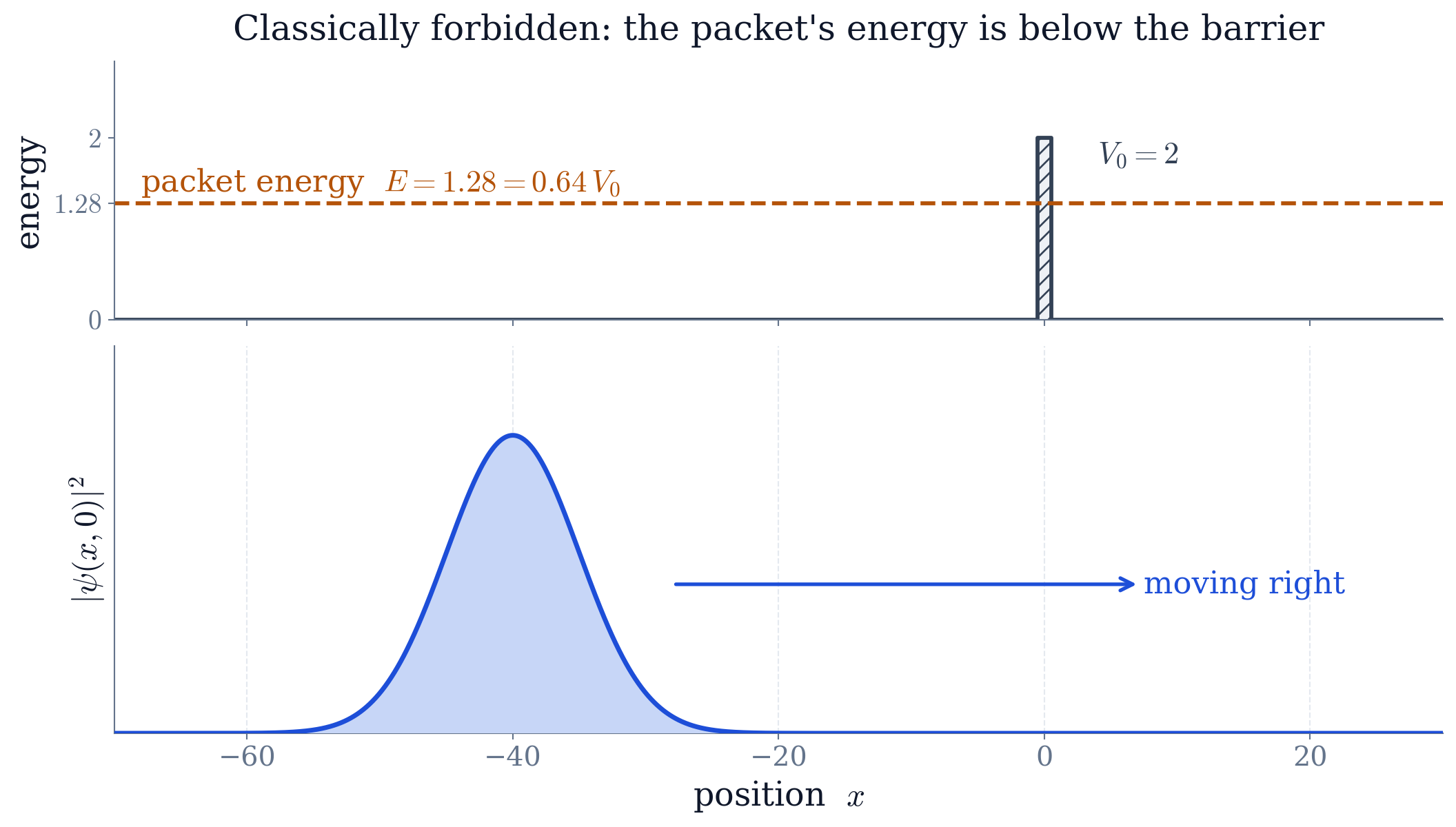
The initial packet and the barrier are shown in Figure 1. The parameters are chosen so that the packet is far from the barrier initially and has a narrow momentum spread (the width $\sigma=5$ gives $\Delta k \approx 0.1$ , small compared to $$k_0=1.6$$ ), ensuring it behaves like a well-defined energy.

Top: the potential, with the packet's mean energy E=1.28 marked against the barrier height V0=2. Bottom: the initial probability density, a Gaussian centred at x0=-40 and moving right. The two panels are kept separate because energy and probability density have different units and cannot honestly share one axis. — Figure 1. Top: the potential, with the packet's mean energy $$E=1.28$$ marked against the barrier height $$V_0=2$$ . Bottom: the initial probability density, a Gaussian centred at $$x_0=-40$$ and moving right. The two panels are kept separate because energy and probability density have different units and cannot honestly share one axis.

5Results

5.1Time evolution

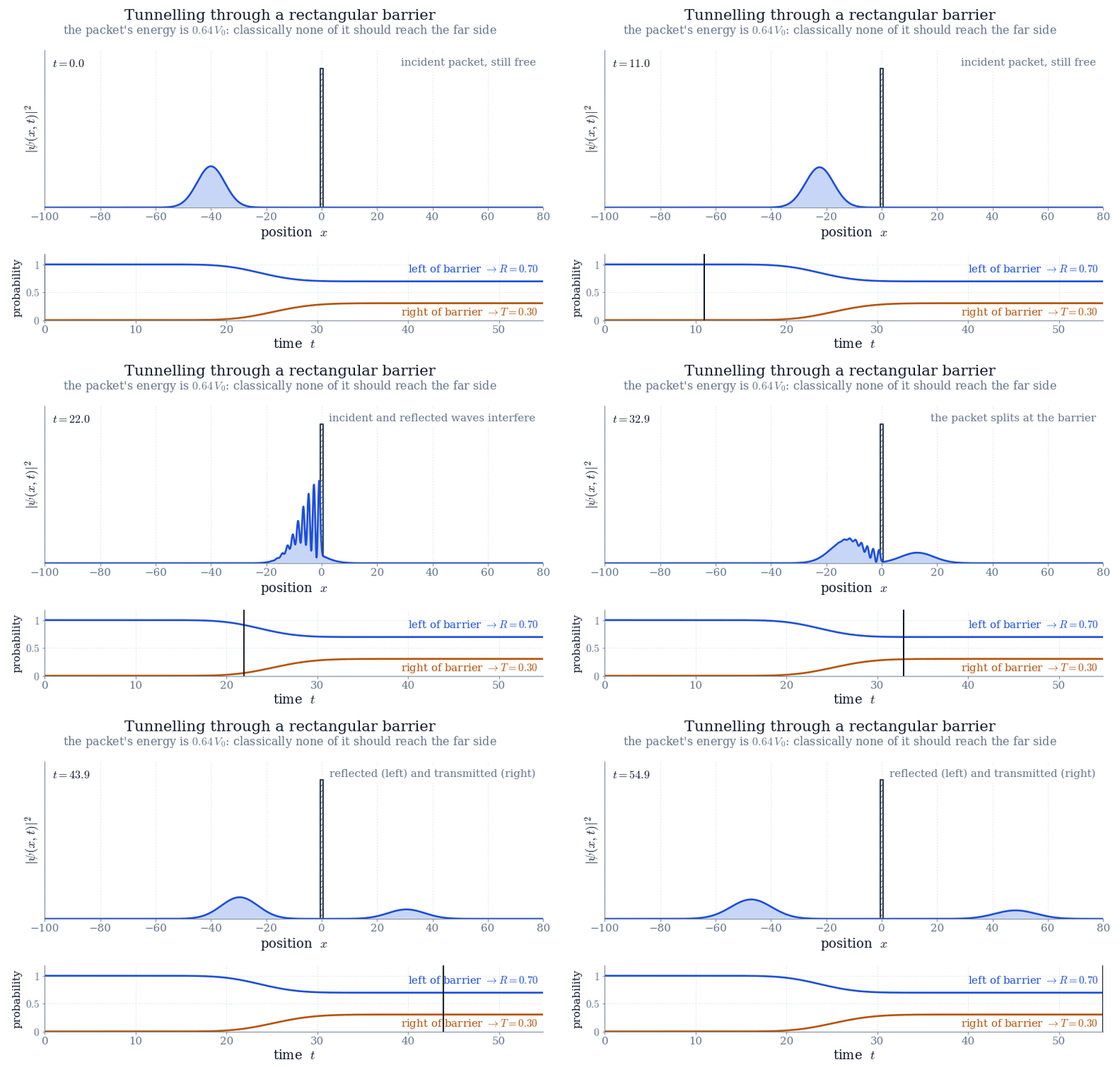
Figure 2 shows $|\psi(x,t)|^2$ as the packet moves right, strikes the barrier, and splits into a reflected part travelling back to the left and a transmitted part continuing to the right.

Time evolution of the probability density |(x,t)|^2 from t=0 to t=55. The packet approaches the barrier (hatched), ripples as the incident and reflected waves interfere on top of one another, and then separates into two pieces moving in opposite directions. The strip underneath integrates ||^2 on each side of the barrier as the collision happens, so the two curves become R and T rather than being quoted at the end: nothing crosses until the packet arrives near t=20, the transfer is over by t 35, and the two levels are flat afterwards because the pieces have separated for good. — Figure 2. Time evolution of the probability density $|\psi(x,t)|^2$ from $$t=0$$ to $$t=55$$ . The packet approaches the barrier (hatched), ripples as the incident and reflected waves interfere on top of one another, and then separates into two pieces moving in opposite directions. The strip underneath integrates $|\psi|^2$ on each side of the barrier as the collision happens, so the two curves *become* $$R$$ and $$T$$ rather than being quoted at the end: nothing crosses until the packet arrives near $$t=20$$ , the transfer is over by $t \approx 35$ , and the two levels are flat afterwards because the pieces have separated for good.

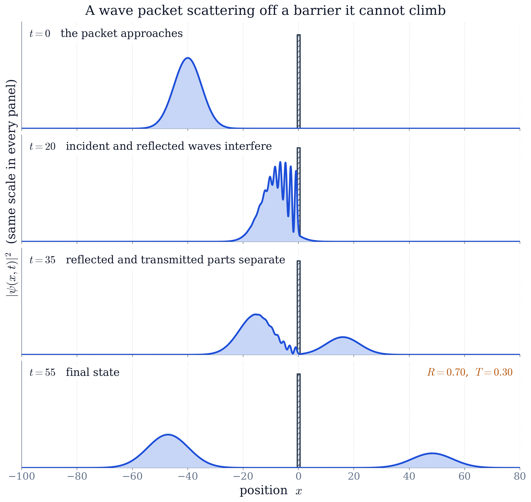
The same evolution is shown as four snapshots in Figure 3. At $$t=22$$ the incident and reflected waves overlap at the barrier and interfere, producing the ripples in the second panel — a purely wave phenomenon with no classical analogue. The interference pattern is a direct consequence of the superposition of the incident and reflected waves, both of which are complex exponentials in the region left of the barrier. By $$t=55$$ the two pieces are cleanly separated: the reflected packet moves left, the transmitted packet moves right.

Snapshots of ||^2 at four selected times. Top to bottom: the incident packet approaching; the moment of interaction, showing incident/reflected interference; the reflected and transmitted parts separating; and the final state with a large reflected packet (left) and a smaller transmitted packet (right). The barrier region is shaded grey. — Figure 3. Snapshots of $|\psi|^2$ at four selected times. Top to bottom: the incident packet approaching; the moment of interaction, showing incident/reflected interference; the reflected and transmitted parts separating; and the final state with a large reflected packet (left) and a smaller transmitted packet (right). The barrier region is shaded grey.

5.2Reflection and transmission probabilities

Integrating the final probability density on each side of the barrier gives

\begin{equation} R = \!\!\int_{x<-a/2}\!\! |\psi|^2\,dx = 0.70, \qquad T = \!\!\int_{x>+a/2}\!\! |\psi|^2\,dx = 0.30, \qquad R+T = 1.00 . \label{eq:RT} \end{equation}

That $$R+T = 1$$ to three digits is an important check: the split-step method is unitary (the evolution operator is a product of unitary operators), so it conserves total probability exactly up to machine precision. The only leak is the absorbing mask at the domain edges; the program prints the running norm, and it stays within $2\times10^{-4}$ of unity for the whole run.

5.3Comparison with analytic theory

For a steady stream of particles of a single energy $$E<V_0$$ , the analytic transmission coefficient of a rectangular barrier is obtained by solving the stationary Schrödinger equation:

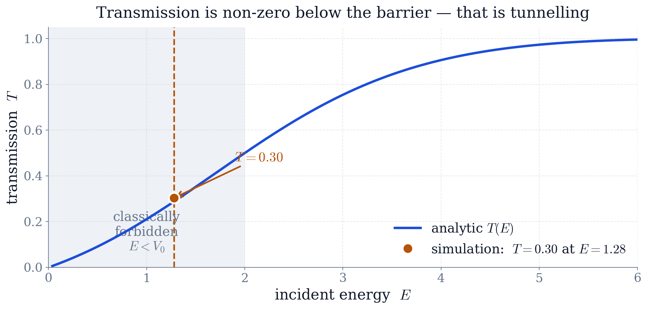
\begin{equation} T(E) = \left[\,1 + \frac{V_0^{2}\,\sinh^{2}(\kappa a)}{4E(V_0-E)}\,\right]^{-1}, \qquad \kappa = \sqrt{2m(V_0 - E)}/\hbar . \label{eq:Tanalytic} \end{equation}

The hyperbolic function $\sinh$ here is exactly the kind that appears when a solution decays inside a classically forbidden region (Chapter 2), and the same formula with $\sinh\to\sin$ holds for $$E>V_0$$ (above-barrier transmission, which shows oscillatory resonances). Figure 4 plots $$T(E)$$ and marks our packet. Evaluated at the mean energy the formula gives $$T(E_0)=0.29$$ , against the measured $$T=0.30$$ — agreement to about $5\%$ , which is as close as one should expect, since the packet is not a single energy but a narrow spread of them. The wave packet, which is a spread of energies around $$E=1.28$$ with width $\Delta E \approx k_0 \Delta k \approx 0.16$ (since $\Delta k \approx 1/(2\sigma)=0.1$ ), behaves as the single-energy theory predicts because the transmission varies slowly over that energy range.

Analytic transmission coefficient T(E) for the barrier (green). The shaded region E<V0 is classically forbidden, yet T>0 there — this is tunnelling. The red dot is the transmission measured from the wave-packet simulation, which agrees with the analytic value at the mean packet energy. — Figure 4. Analytic transmission coefficient $$T(E)$$ for the barrier (green). The shaded region $$E<V_0$$ is classically forbidden, yet $$T>0$$ there — this is tunnelling. The red dot is the transmission measured from the wave-packet simulation, which agrees with the analytic value at the mean packet energy.

5.4Convergence and error analysis

To verify the numerical accuracy, we performed convergence tests:

Time-step convergence: Reducing $\Delta t$ from $$0.004$$ to $$0.002$$ changed $$T$$ by less than $0.2\%$ .
Spatial resolution: Doubling $$N$$ from $$8192$$ to $$16384$$ changed $$T$$ by $0.1\%$ .
Total probability conservation: The quantity $\int |\psi|^2 dx$ stayed within $2\times10^{-4}$ of unity for the whole run — the program prints this figure — and before the absorbing mask is applied it is conserved exactly.

These tests confirm that the chosen parameters are sufficient for the accuracy reported. The full program is code/make\_figures.py; running it inside code/ reproduces every figure here along with the printed values of $$R$$ , $$T$$ and the running norm.

6Discussion: which course methods were used

Every step of this project used a tool from the course:

Complex numbers (Chapter 2). The wavefunction is complex, the packet's momentum enters through the phase $e^{ik_0x}$ , and every step of the algorithm multiplies by a complex exponential. The $\sinh$ in the transmission formula is the complex exponential seen along the “forbidden” direction.
Fourier transforms (Chapter 7). The split-step method works only because the kinetic operator is diagonal in Fourier space; the FFT is what makes each time step cheap. Writing the packet as a superposition of plane waves is a Fourier decomposition.
Partial differential equations (Chapter 10). The Schrödinger equation is a PDE, and the split-step method is one practical way to integrate it in time, complementing the separation-of-variables approach of that chapter. The concept of unitary evolution also ties to the spectral theory of differential operators.

The physics conclusion is that a particle really can cross a barrier it lacks the energy to surmount, with a probability that drops sharply as the barrier gets higher or wider (through the $\sinh^2(\kappa a)$ factor). The mathematics conclusion is that a short, transparent program built from Fourier transforms and complex exponentials reproduces the exact result and, unlike the plane-wave formula, lets us watch the process happen.

7Conclusion

We solved the 1D time-dependent Schrödinger equation for a wave packet incident on a rectangular barrier using the split-step Fourier method. With the packet's energy at $0.64\,V_0$ we found $$R=0.70$$ and $$T=0.30$$ , conserving probability and matching the analytic transmission coefficient. The project shows tunnelling directly and demonstrates how the course's methods — complex exponentials, the Fourier transform, and the PDE viewpoint — combine into a single working calculation.

The split-step Fourier method is versatile and can be extended to more complex potentials and higher dimensions. It also illustrates the deep connection between operator splitting and the Baker–Campbell–Hausdorff formula, a topic that appears in advanced quantum mechanics. This project thus serves as both a concrete application of course material and a stepping stone to more sophisticated simulations.

References

D. J. Griffiths, Introduction to Quantum Mechanics, Cambridge University Press, 3rd ed., 2018.
M. L. Boas, Mathematical Methods in the Physical Sciences, Wiley, 3rd ed., 2006.
R. W. Hamming, Numerical Methods for Scientists and Engineers, Dover, 1986 (for split-step methods).

Acknowledgments

The author thanks the PHYS 3260 teaching team for providing the course framework and the initial project template. The Python implementation uses NumPy and Matplotlib, which are open-source libraries.

← All projects