Worked example · solved on paper

Why a Drum Has No Pitch: Modes of a Circular Membrane

PHYS 3260, Mathematical Methods — worked example

The problem

A drumhead of radius $$R$$ is a membrane held at tension $\tau$ with areal density $\sigma$ , clamped so that its rim cannot move. Its small transverse displacements $\psi(r,\theta,t)$ satisfy the two-dimensional wave equation with a fixed boundary,

\frac{\partial ^2\psi}{\partial t^2} = c^2\nabla^2\psi , \qquad \psi(R,\theta,t) = 0 , \qquad c = \sqrt{\tau/\sigma} .

(a)
Separate the variables in polar coordinates. Show that the radial factor obeys Bessel's equation, and use the clamped rim together with regularity at the centre to obtain the normal modes of the drumhead and their frequencies $\omega_{nm}$ .
(b)
Show that the $\omega_{nm}$ are not integer multiples of the lowest of them, and account for what that does to the sound: why a plucked string has a pitch and a struck drum has not.
(c)
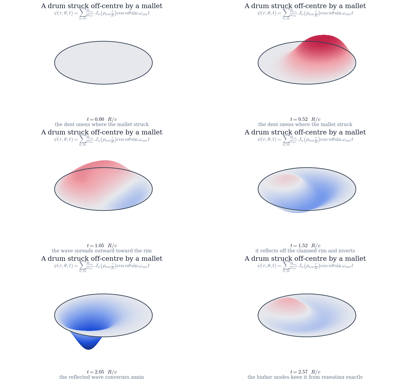
The drum is struck off centre. At $$t=0$$ the membrane is flat but carries a localised patch of upward velocity. Expand that initial condition in the modes of (a), state the orthogonality relation the expansion relies on, and animate the motion that follows.

Abstract. The wave equation on a disc with a clamped rim is separated in polar coordinates, which turns the radial part into Bessel's equation. The rim condition then selects the zeros $\rho_{nm}$ of $$J_n$$ , and the mode frequencies come out as $\omega_{nm} = c\,\rho_{nm}/R$ . Because those zeros are not evenly spaced, a drum's overtones are not integer multiples of its fundamental — the reason a drum sounds like a drum and not like a string. The modes are then used as a basis: a mallet strike is expanded in them with the Fourier–Bessel orthogonality relation, and the resulting sum is animated to show the membrane moving. The work draws on series solutions of differential equations (Ch. 9), partial differential equations (Ch. 10), orthogonal expansions (Ch. 7) and integration in polar coordinates (Ch. 5).

1The physics question

Strike a guitar string and you hear a note. Strike a drum and you hear a thud: loud, definite, but hard to sing back. The difference is not in how the two are played but in the shape of the boundary that holds them. A string is clamped at two points and vibrates at frequencies $f, 2f, 3f, \dots$ ; those integer multiples are what the ear fuses into a pitch. A drumhead is clamped around a circle, and this project works out what that circular boundary allows.

Parts (a) and (b) settle what that boundary allows and what the ear then makes of it. Part (c) is the harder half, and the one a real drum poses: a mallet does not set a single mode going, so the motion you actually see has to be assembled out of all of them.

2The mathematical model

Let $\psi(r,\theta,t)$ be the vertical displacement of a membrane of radius $$R$$ , held fixed at the rim. Small transverse vibrations obey the two-dimensional wave equation

\begin{equation} \frac{\partial ^2 \psi}{\partial t^2} = c^2 \nabla^2 \psi, \label{eq:wave} \end{equation}

where $c = \sqrt{\tau/\sigma}$ is set by the tension $\tau$ and the areal density $\sigma$ . The geometry is circular, so the Laplacian is used in polar coordinates,

\begin{equation} \nabla^2 \psi = \frac{1}{r}\frac{\partial}{\partial r}\!\left( r\,\frac{\partial \psi}{\partial r} \right) + \frac{1}{r^2}\,\frac{\partial ^2 \psi}{\partial \theta^2}. \label{eq:laplacian} \end{equation}

The boundary condition is that the rim never moves,

\begin{equation} \psi(R, \theta, t) = 0 \quad\text{for all } \theta, t, \label{eq:bc} \end{equation}

and the solution must also be finite and single-valued at every interior point, including the centre $$r = 0$$ where $\eqref{eq:laplacian}$ is singular. That regularity requirement is not a technicality: it is what removes half of the solutions below.

Throughout the calculations $$R = c = 1$$ , so frequencies are quoted in units of $$c/R$$ and lengths in units of $$R$$ .

3Separating the variables (Chapter 10)

This is the method of Chapter 10 applied to a circular boundary. Look for solutions of the product form

\begin{equation} \psi(r,\theta,t) = P(r)\,\Theta(\theta)\,T(t). \end{equation}

Substituting into $\eqref{eq:wave}$ and dividing by $P\Theta T$ gives

\begin{equation} \frac{1}{c^2}\frac{T''}{T} = \frac{1}{P}\left( P'' + \frac{1}{r}P' \right) + \frac{1}{r^2}\frac{\Theta''}{\Theta}. \end{equation}

The left side depends only on $$t$$ and the right side only on $$r$$ and $\theta$ , so both equal a constant. Calling it $$-k^2$$ — negative, because a positive constant would give solutions growing without bound in time, which a membrane with a fixed rim cannot do — gives

\begin{equation} T'' + \omega^2 T = 0, \qquad \omega = c\,k . \label{eq:time} \end{equation}

Separating $$r$$ from $\theta$ in the remainder introduces a second constant,

\begin{equation} \frac{\Theta''}{\Theta} = -n^2 , \qquad r^2 P'' + r P' + \left( k^2 r^2 - n^2 \right) P = 0 . \label{eq:radial} \end{equation}

3.1The angular equation

The solution of $\Theta'' + n^2\Theta = 0$ is $\Theta(\theta) = A\cos n\theta + B\sin n\theta$ . Going once around the membrane must return to the same displacement, $\Theta(\theta + 2\pi) = \Theta(\theta)$ , which forces $$n$$ to be an integer. The integer $$n$$ counts nodal diameters: straight lines across the drumhead that never move. Taking the strike to lie on the $$x$$ -axis makes the motion symmetric about that line, so only the $\cos n\theta$ terms are needed below.

3.2The radial equation: Bessel's equation (Chapter 9)

Equation $\eqref{eq:radial}$ is Bessel's equation of order $$n$$ in the variable $$kr$$ . It has a regular singular point at $$r=0$$ , so it is solved by the Frobenius series of Chapter 9 rather than by an ordinary power series. Its general solution is

\begin{equation} P(r) = C\,J_n(kr) + D\,Y_n(kr), \end{equation}

where $$J_n$$ and $$Y_n$$ are the Bessel functions of the first and second kind — exactly the functions Chapter 9 obtains by solving $\eqref{eq:radial}$ as a power series about the regular singular point $$r=0$$ . Since $Y_n(kr) \to -\infty$ as $r \to 0$ and a real drumhead has a finite displacement at its centre, $$D = 0$$ .

3.3The clamped rim quantises the frequency

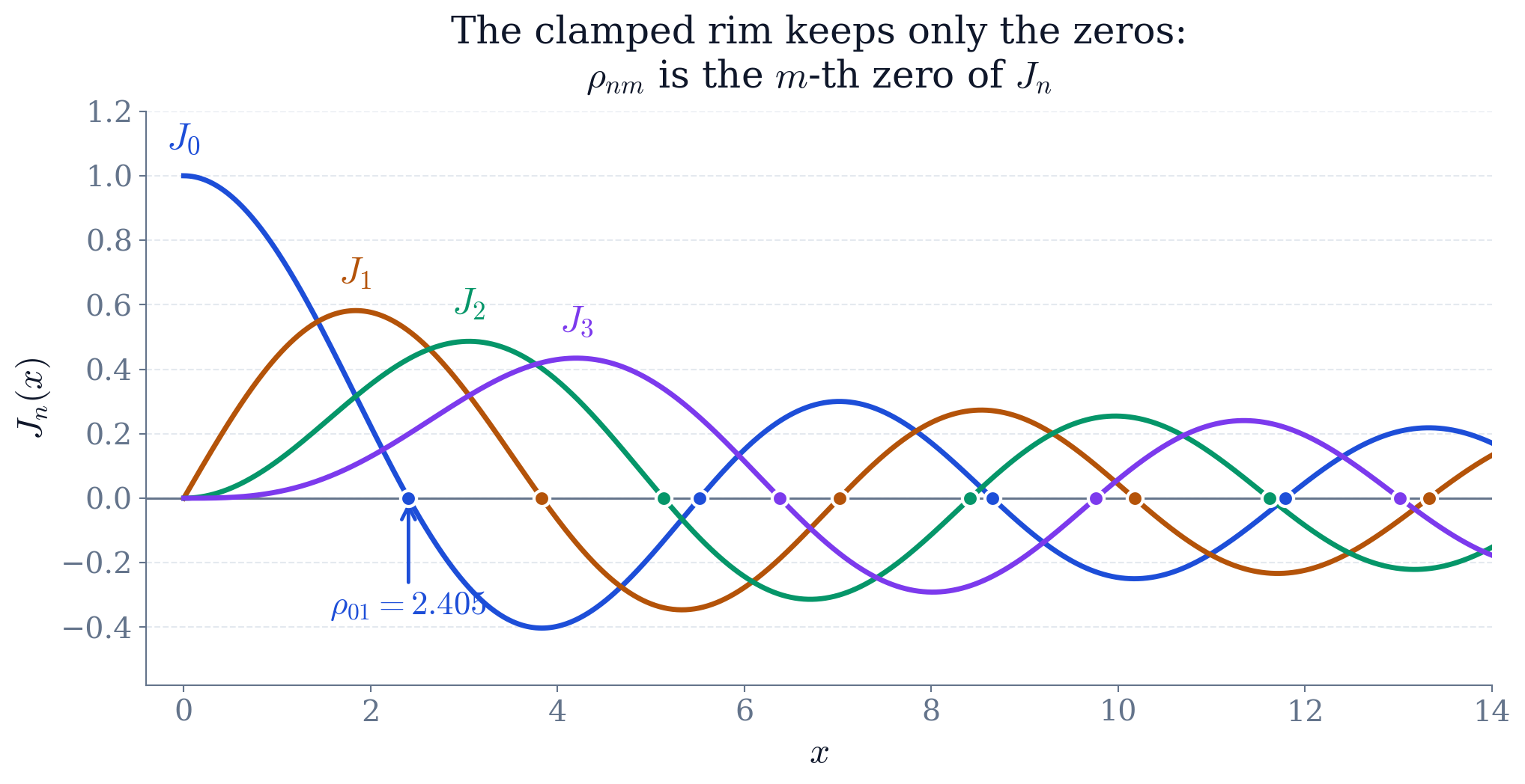
The boundary condition $\eqref{eq:bc}$ now bites: $$J_n(kR) = 0$$ , so $$kR$$ must be a zero of $$J_n$$ . Writing $\rho_{nm}$ for the $$m$$ -th positive zero of $$J_n$$ (Figure 1),

\begin{equation} k_{nm} = \frac{\rho_{nm}}{R}, \qquad \boxed{\;\omega_{nm} = \frac{c\,\rho_{nm}}{R}\;} \label{eq:omega} \end{equation}

This is the same logic as a string, where the fixed ends force $\sin(kL)=0$ and hence $k = m\pi/L$ . The difference is entirely in which function has to vanish: $\sin$ for the string, $$J_n$$ for the drum.

The first four Bessel functions of the first kind. The dots mark their zeros nm, and those are the only radial wavenumbers a clamped circular rim allows. Unlike the zeros of , they are not evenly spaced — and their spacing is not the same from one Jn to the next. — Figure 1. The first four Bessel functions of the first kind. The dots mark their zeros $\rho_{nm}$ , and those are the only radial wavenumbers a clamped circular rim allows. Unlike the zeros of $\sin$ , they are not evenly spaced — and their spacing is not the same from one $$J_n$$ to the next.

3.4The normal modes

Collecting the three factors, the normal modes of the drumhead are

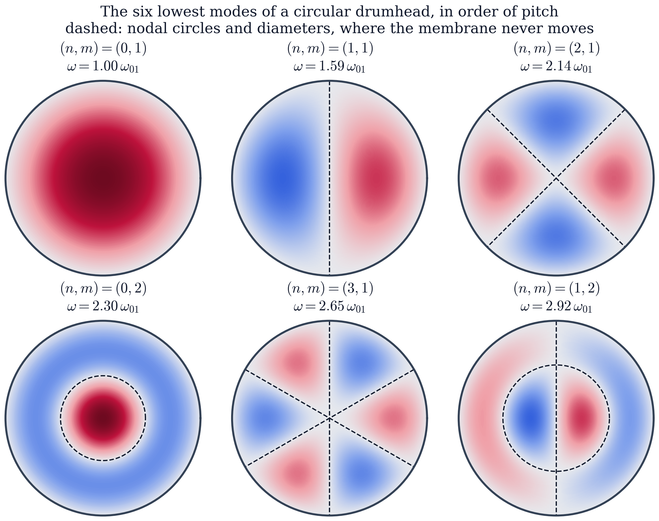
\begin{equation} \psi_{nm}(r,\theta,t) = J_n\!\left( \rho_{nm}\frac{r}{R} \right)\cos(n\theta)\, \left[\, a_{nm}\cos \omega_{nm} t + b_{nm}\sin \omega_{nm} t \,\right], \qquad n \ge 0,\; m \ge 1 . \label{eq:modes} \end{equation}

Each mode has $$n$$ nodal diameters and $$m-1$$ interior nodal circles, the circles sitting at the radii where $J_n(\rho_{nm} r/R)$ passes through its earlier zeros. Figure 3 shows the six lowest.

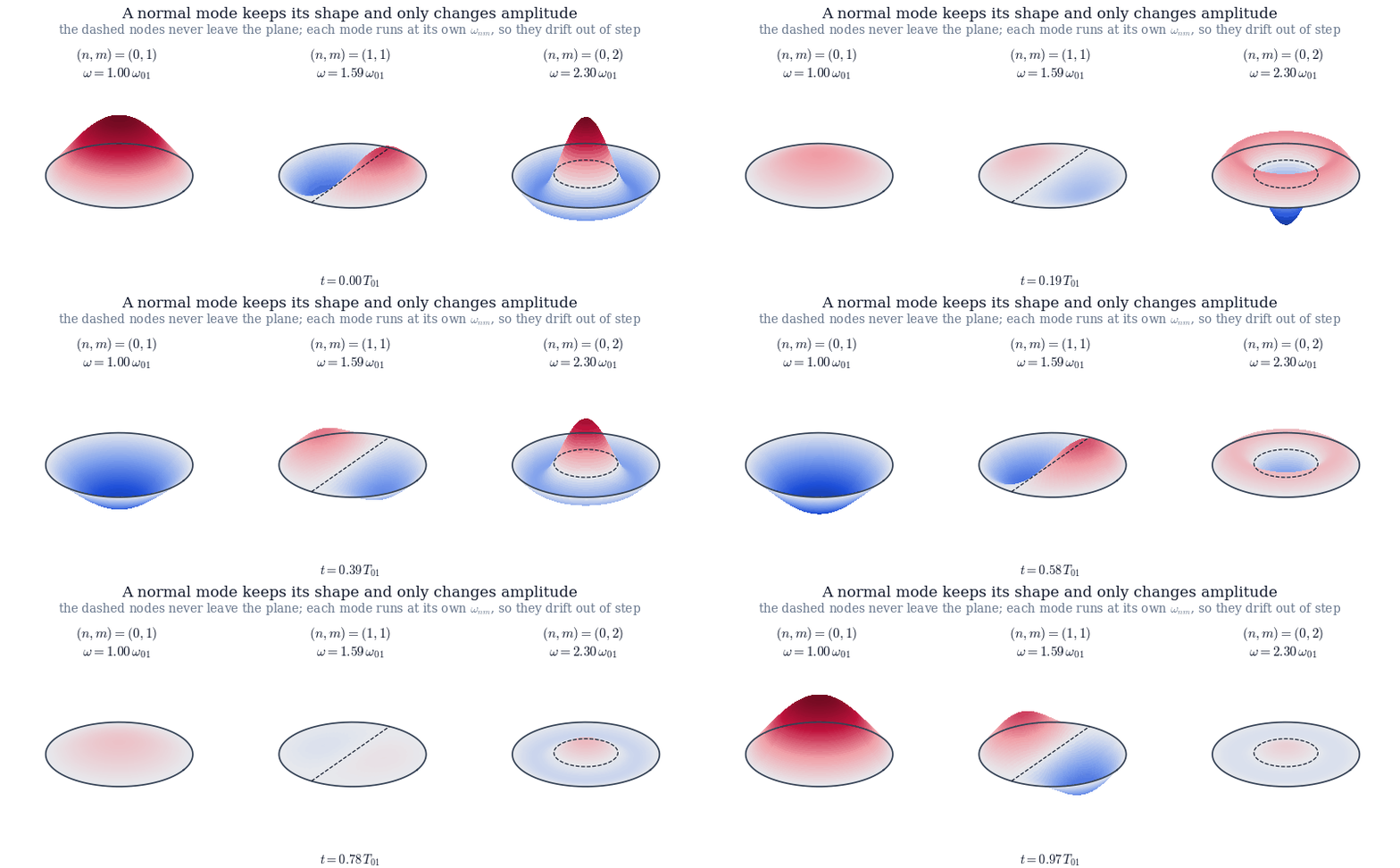
What a normal mode is shows up better in motion than on the page: the pattern is fixed for all time and only its amplitude oscillates, so the nodes never move. Figure 2 runs three modes side by side. Because each carries its own $\omega_{nm}$ , they start together and immediately drift apart — and that drift is the whole reason a struck drum does not repeat itself.

Three normal modes as surfaces, each oscillating at its own frequency: (0,1) at 01, (1,1) at 1.59\,01 and (0,2) at 2.30\,01. The membrane rises and falls, but the shape is fixed: the dashed nodal lines never leave the plane, and every point of the membrane passes through zero at the same instant. After one period of the fundamental the left surface has returned to where it began and the other two have not. — Figure 2. Three normal modes as surfaces, each oscillating at its own frequency: $$(0,1)$$ at $\omega_{01}$ , $$(1,1)$$ at $1.59\,\omega_{01}$ and $$(0,2)$$ at $2.30\,\omega_{01}$ . The membrane rises and falls, but the shape is fixed: the dashed nodal lines never leave the plane, and every point of the membrane passes through zero at the same instant. After one period of the fundamental the left surface has returned to where it began and the other two have not.

The six lowest modes, ordered by frequency rather than by index. Red and blue are opposite directions of displacement; the dashed lines are the nodes, which stay still for all time. The ordering by pitch mixes the two indices: (2,1) is lower than (0,2). — Figure 3. The six lowest modes, ordered by frequency rather than by index. Red and blue are opposite directions of displacement; the dashed lines are the nodes, which stay still for all time. The ordering by pitch mixes the two indices: $$(2,1)$$ is lower than $$(0,2)$$ .

4Why the drum has no pitch

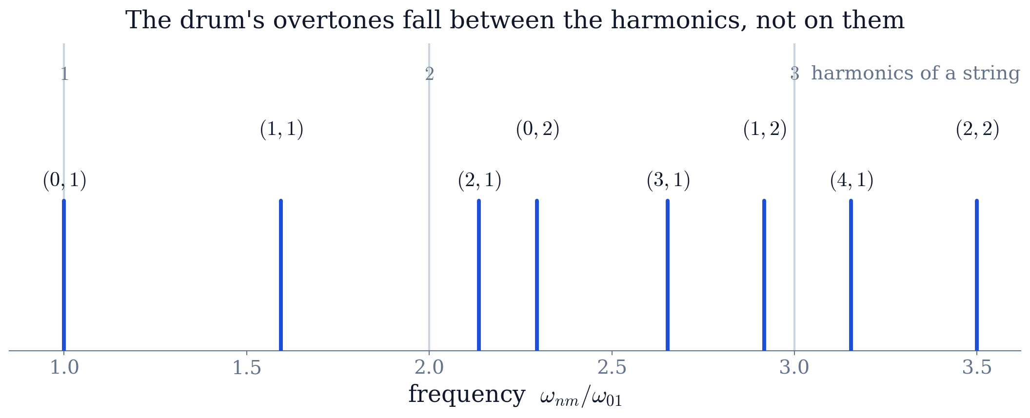
The frequencies $\eqref{eq:omega}$ in units of the fundamental $\omega_{01}$ are

\begin{equation} \frac{\omega_{nm}}{\omega_{01}} = \frac{\rho_{nm}}{\rho_{01}} = 1,\; 1.593,\; 2.136,\; 2.295,\; 2.653,\; 2.917,\; \dots \label{eq:ratios} \end{equation}

and not one of them after the first is an integer. A string would give $1, 2, 3, 4, \dots$ . The ear reads an integer series as a single note with a timbre; a non-integer series it reads as a noise with a rough centre of gravity. That is the whole difference between a drum and a string, and it comes from the spacing of the zeros of $$J_n$$ — from the geometry of the boundary, not from the material of the membrane. Figure 4 puts the two ladders side by side.

Figure 4. The eight lowest drum frequencies against the harmonic series a string would produce (grey). Only the fundamental lands on a harmonic.

All of this is an argument about hearing, made on paper. The panel below settles it by ear. Both sounds are built from the modes derived above — one partial per $\omega_{nm}$ , each given the amplitude the mallet delivers to that mode — and the second is the same mallet striking a clamped string as long as the drum is wide, hit the same distance off centre. The two are then transposed to a common fundamental, so that the one difference left between them is the ladder $\eqref{eq:ratios}$ against $1, 2, 3, \dots$ .

Listen The same mallet on two boundaries

Interactive visualization placeholder.

Seven seconds of each, and the button plays them back to back, since a difference in pitch is far easier to name across four seconds than across half a minute. The circular rim gives a thud the ear cannot pin a note to: with partials at $1, 1.59, 2.14, 2.30, \dots$ there is no fundamental they all belong to. The two fixed ends give a note, because $1, 2, 3, \dots$ is the pattern the ear fuses into a single pitch. Both sounds are matched in loudness and transposed to the same fundamental, so neither of those can be what you are hearing. The amplitudes are the Fourier–Bessel coefficients of Figure 5, weighted by $\omega_{nm}$ because a source small compared with a wavelength radiates in proportion to its acceleration; the damping is lighter than a real drumhead's, so that there is something left to listen to after seven seconds.

A second feature of $\eqref{eq:ratios}$ is worth naming: every mode with $n \ge 1$ is doubly degenerate. Replacing $\cos n\theta$ by $\sin n\theta$ gives a different pattern — the same shape rotated by half a nodal sector — at exactly the same frequency. Which of the pair is excited depends only on where the drum is struck.

5Striking the drum: an initial-value problem

Equation $\eqref{eq:modes}$ describes what the membrane can do. What it actually does is fixed by how it is started. A drum is struck, not plucked: the mallet leaves the membrane flat but moving,

\begin{equation} \psi(r,\theta,0) = 0, \qquad \left.\frac{\partial \psi}{\partial t}\right|_{t=0} = v(r,\theta), \label{eq:ic} \end{equation}

with $$v$$ a localised patch of velocity where the mallet landed. Here $$v$$ is a Gaussian of width $$0.24R$$ centred at $$r = 0.4R$$ on the $$x$$ -axis.

The initial displacement being zero kills every $a_{nm}$ in $\eqref{eq:modes}$ , leaving

\begin{equation} \psi(r,\theta,t) = \sum_{n,m} \frac{B_{nm}}{\omega_{nm}}\, J_n\!\left( \rho_{nm}\frac{r}{R} \right)\cos(n\theta)\, \sin(\omega_{nm} t), \label{eq:solution} \end{equation}

where the $B_{nm}$ are the coefficients of $$v$$ in the mode basis. Finding them is an orthogonal expansion of exactly the kind Chapter 7 performs with sines and cosines — the only differences are that the basis functions are Bessel functions instead of sinusoids and that the inner product carries a weight. The modes are orthogonal on the disc under

\begin{equation} \langle u, w \rangle = \int_0^{R}\!\!\int_0^{2\pi} u\,w\; r\,d\theta\,dr, \label{eq:inner} \end{equation}

in which the factor $$r$$ is the Jacobian of polar coordinates (Chapter 5) and is what makes the orthogonality work. Projecting,

\begin{equation} B_{nm} = \frac{\langle v,\, \psi_{nm}\rangle}{\langle \psi_{nm},\, \psi_{nm}\rangle}. \label{eq:coefficients} \end{equation}

This is the Fourier–Bessel series, the circular counterpart of a Fourier sine series.

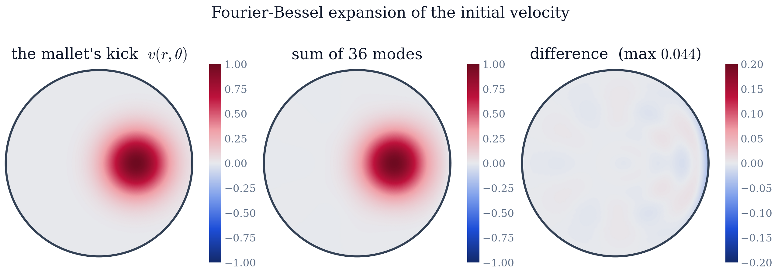
Figure 5 checks the expansion: 36 modes ( $n \le 5$ , $m \le 6$ ) reproduce the strike to within $4.4\%$ of its peak. The error is concentrated at the sharp edge of the patch, as it always is when a truncated orthogonal series meets a steep feature.

Figure 5. The mallet's velocity patch (left), the sum of 36 modes fitted to it (centre), and the difference (right, on a five-times finer colour scale). The residual sits at the rim of the patch, where the truncated series cannot follow the sharp gradient.

The factor $1/\omega_{nm}$ in $\eqref{eq:solution}$ is worth a comment. A kick of a given size sets a stiff, high-frequency mode swinging through a smaller displacement than a floppy one, so the visible motion is dominated by the lowest few modes even though the strike deposits energy across many. This is why Figure 6 stays smooth despite starting from a sharply localised strike.

Figure 6. The struck membrane over one period of the fundamental. The dent from the mallet spreads outward, reflects off the clamped rim, and returns; the higher modes ride on top of the fundamental at their own, unrelated, frequencies, so the surface never repeats exactly.

6Which course methods were used

Series solutions of differential equations (Chapter 9). The radial equation $\eqref{eq:radial}$ is Bessel's equation; $$J_n$$ and $$Y_n$$ are its two series solutions about the regular singular point at the origin, and discarding $$Y_n$$ on grounds of regularity is the step that halves the solution space.
Partial differential equations (Chapter 10). Separation of variables turns one PDE in three variables into three ordinary differential equations, and the boundary conditions — periodicity in $\theta$ , regularity at $$r=0$$ , clamping at $$r=R$$ — are what quantise $$n$$ and $\omega_{nm}$ .
Fourier series and orthogonal expansions (Chapter 7). The Fourier–Bessel expansion $\eqref{eq:coefficients}$ is the same projection onto an orthogonal basis, with $$J_n$$ in place of sines and the weight $$r$$ in the inner product.
Multiple integrals (Chapter 5). The inner product $\eqref{eq:inner}$ is an area integral in polar coordinates, and the factor $$r$$ in it is the Jacobian.

7Conclusion

Separating the wave equation on a disc gives modes $J_n(\rho_{nm}r/R)\cos(n\theta)$ with frequencies $\omega_{nm} = c\rho_{nm}/R$ , where the $\rho_{nm}$ are the zeros of the Bessel functions. Those zeros are not evenly spaced, so the overtones are not harmonics — the drum has a sound but no pitch, and the reason is the shape of its boundary. Treating the modes as a basis then solves the real problem: a strike is expanded in them by Fourier–Bessel projection, and the resulting sum reproduces the visible motion of a struck drumhead.

The same machinery carries over unchanged to a circular waveguide, a vibrating plate, or the orbitals of the hydrogen atom: whenever the boundary is circular or spherical, separation of variables produces a special function whose zeros the boundary condition selects.

References

M. L. Boas, Mathematical Methods in the Physical Sciences, Wiley, 3rd ed., 2006 (Chapters 12 and 13).
P. M. Morse, Vibration and Sound, McGraw–Hill, 2nd ed., 1948 (the circular membrane and its inharmonicity).
SciPy documentation, scipy.special.jv and scipy.special.jn\_zeros.

← All projects