Worked example · solved on paper

A Standing Electromagnetic Wave in a Square Cavity

PHYS 3260, Mathematical Methods — worked example

The problem

Consider the electromagnetic field

\begin{equation} \vec{E}(x, y, t) = E_0 \cos\!\left( \frac{\pi x}{L} \right) \cos\!\left( \frac{\pi y}{L} \right) \sin(\omega t)\, \hat{\mathbf{k}}, \label{eq:Egiven} \end{equation}

\begin{equation} \vec{B}(x, y, t) = B_0 \left[ - \cos\!\left( \frac{\pi x}{L} \right) \sin\!\left( \frac{\pi y}{L} \right) \hat{\mathbf{i}} + \sin\!\left( \frac{\pi x}{L} \right) \cos\!\left( \frac{\pi y}{L} \right) \hat{\mathbf{j}} \right] \cos(\omega t). \label{eq:Bgiven} \end{equation}

(a)
Show that this field satisfies Maxwell's equations in vacuum if
$\omega = \frac{\sqrt{2}\, \pi c}{L}, \qquad B_0 = \frac{E_0}{\sqrt{2}\,c}.$
(b)
The field is a standing electromagnetic wave inside a metal-walled cavity of square cross-section $L \times L$ parallel to the $$xy$$ -plane and very long in the $$z$$ -direction — a cavity oscillator. Sketch $\vec{E}$ and $\vec{B}$ . The wave number is $k = \pi/L$ , so the wavelength is $\lambda = 2L$ .

Abstract. A pair of fields is proposed for the inside of a long metal-walled pipe of square cross-section. Requiring that they satisfy Maxwell's equations in vacuum fixes both the oscillation frequency, $\omega = \sqrt{2}\,\pi c/L$ , and the ratio of the field amplitudes, $B_0 = E_0/(\sqrt{2}c)$ . Separating variables in the resulting wave equation then produces the whole family of allowed modes, $\omega_{mn} = (\pi c/L)\sqrt{m^2+n^2}$ , of which the given field is the lowest. Python turns the closed-form fields into maps of $\vec{E}$ and $\vec{B}$ and into an animation, which shows the electric and magnetic energy trading places twice per period. The work uses partial differentiation and the vector operators of Chapter 6 and the separation-of-variables method for partial differential equations of Chapter 10.

1The physics question

The problem hands over a pair of fields and asks whether they can exist. That is a shorter road to the same physics than solving Maxwell's equations from nothing: substituting $\eqref{eq:Egiven}$ and $\eqref{eq:Bgiven}$ into the four equations turns each of them into an algebraic condition, and two of those conditions are what fix the only unknowns in the problem, $\omega$ and $$B_0$$ . Part (b) then names what the algebra has produced — the lowest standing-wave mode of a hollow metal pipe of square cross-section — and this report takes that one step past what was asked, separating variables in the wave equation to get the whole family of modes such a cavity supports, of which the given field is the first.

Throughout, the cross-section is centred on the origin, so $$x$$ and $$y$$ each run over $[-L/2,\, L/2]$ . That choice matters: $\cos(\pi x/L)$ vanishes at $x = \pm L/2$ , which is exactly the boundary condition a conducting wall imposes. Written on a $$[0, L]$$ grid the same formula would put a maximum on the wall and would not be a cavity field at all.

2Maxwell's equations and the boundary conditions

In a linear medium Maxwell's equations read

\begin{align} \nabla \cdot \vec{D} &= \rho_f, & \nabla \times \vec{E} &= -\frac{\partial \vec{B}}{\partial t}, \notag \\ \nabla \cdot \vec{B} &= 0, & \nabla \times \vec{H} &= \vec{J}_f + \frac{\partial \vec{D}}{\partial t}, \label{eq:maxwell-medium} \end{align}

where $\rho_f$ is the free charge density and $\vec{J}_f$ the free current density, and where

\begin{equation} \vec{D} = \varepsilon_0 \vec{E} + \vec{P}, \qquad \vec{B} = \mu_0 (\vec{H} + \vec{M}), \end{equation}

with $\vec{P}$ the polarisation (electric dipole moment per unit volume) and $\vec{M}$ the magnetisation (magnetic dipole moment per unit volume).

2.1Boundary conditions at an interface

Let $\mathcal{S}$ separate two homogeneous isotropic media, and let $\hat{\mathbf{n}}$ be the unit normal pointing from medium 1 into medium 2. Applying the integral form of $\eqref{eq:maxwell-medium}$ to a flat pillbox and to a vanishing-height loop straddling the surface gives the four matching conditions. The two integral theorems used below — the divergence theorem for the pillboxes and Stokes' theorem for the loops — are the ones proved in Chapter 6; here they do the work of turning differential equations into statements about what happens at a surface.

Gauss's law on a thin pillbox gives

\begin{equation} \oint \vec D\cdot d\vec S = Q_{\mathrm{f}} \;\Longrightarrow\; (\vec D_2 - \vec D_1)\cdot\hat{\mathbf n}\,\Delta S = \sigma_f\,\Delta S, \label{eq:pillbox} \end{equation}

and the same pillbox applied to $\oint \vec B\cdot d\vec S = 0$ gives the magnetic counterpart. Faraday's law on a rectangular loop of length $\Delta\ell$ whose height goes to zero encloses no flux, so

\begin{equation} \oint_{\ell} \vec E\cdot d\vec l = -\frac{d}{dt}\int_S \vec B\cdot d\vec S \approx 0, \label{eq:loop} \end{equation}

and the Ampère–Maxwell law on that loop encloses only the surface current. Together, $\eqref{eq:pillbox}$ and $\eqref{eq:loop}$ give the four matching conditions

\begin{align} \hat{\mathbf n}\cdot(\vec D_2-\vec D_1) &= \sigma_f, & \hat{\mathbf n}\times(\vec E_2-\vec E_1) &= \vec 0, \notag \\ \hat{\mathbf n}\cdot(\vec B_2-\vec B_1) &= 0, & \hat{\mathbf n}\times(\vec H_2-\vec H_1) &= \vec K_f . \label{eq:bcs} \end{align}

Inside a perfect conductor both fields vanish, so the second and third of $\eqref{eq:bcs}$ say that at the cavity wall the tangential electric field and the normal magnetic field must be zero. For the field $\eqref{eq:Egiven}$ the only component of $\vec E$ is tangential to every wall, which is why $$E_z$$ has to vanish on all four of them.

2.2Reduction to the source-free vacuum equations

Inside the cavity there are no free charges or currents and no matter to polarise: $\rho_f = 0$ , $\vec{J}_f = 0$ , $\vec{P} = \vec{M} = 0$ . Equations $\eqref{eq:maxwell-medium}$ collapse to

\begin{align} \nabla \cdot \vec{E} &= 0, & \nabla \times \vec{E} &= -\frac{\partial \vec{B}}{\partial t}, \notag\\ \nabla \cdot \vec{B} &= 0, & \nabla \times \vec{B} &= \frac{1}{c^2}\frac{\partial \vec{E}}{\partial t}, \label{eq:maxwell-vacuum} \end{align}

with $c = 1/\sqrt{\varepsilon_0 \mu_0}$ .

3(a) Verifying the field

Each of the four equations in $\eqref{eq:maxwell-vacuum}$ is now checked in turn. Every step is a partial derivative of a product of sines and cosines — the machinery of Chapter 6.

3.1Divergence of $\vec{E}$

With $\nabla = \hat{\mathbf{i}}\,\frac{\partial}{\partial x} + \hat{\mathbf{j}}\,\frac{\partial}{\partial y} + \hat{\mathbf{k}}\,\frac{\partial}{\partial z}$ and $\vec{E} = E_z\hat{\mathbf{k}}$ ,

\begin{equation} \nabla \cdot \vec{E} = \frac{\partial E_x}{\partial x} + \frac{\partial E_y}{\partial y} + \frac{\partial E_z}{\partial z} = \frac{\partial E_z}{\partial z} = 0, \label{eq:divE} \end{equation}

because $$E_z$$ does not depend on $$z$$ .

3.2Divergence of $\vec{B}$

Here $$B_z = 0$$ and

\begin{align*} \frac{\partial B_x}{\partial x} &= \frac{\pi}{L} B_0 \sin\!\left( \frac{\pi x}{L} \right) \sin\!\left( \frac{\pi y}{L} \right) \cos(\omega t), \\ \frac{\partial B_y}{\partial y} &= -\frac{\pi}{L} B_0 \sin\!\left( \frac{\pi x}{L} \right) \sin\!\left( \frac{\pi y}{L} \right) \cos(\omega t), \end{align*}

which cancel term by term, so

\begin{equation} \nabla \cdot \vec{B} = \frac{\partial B_x}{\partial x} + \frac{\partial B_y}{\partial y} = 0 . \label{eq:divB} \end{equation}

3.3Curl of $\vec{E}$ : Faraday's law

Since $\vec E$ has only a $$z$$ -component,

\begin{equation} \nabla \times \vec{E} = \frac{\partial E_z}{\partial y}\,\hat{\mathbf{i}} - \frac{\partial E_z}{\partial x}\,\hat{\mathbf{j}}, \label{eq:curlE-general} \end{equation}

and with

\begin{align*} \frac{\partial E_z}{\partial y} &= -E_0 \frac{\pi}{L} \cos\!\left( \frac{\pi x}{L} \right) \sin\!\left( \frac{\pi y}{L} \right) \sin(\omega t), \\ \frac{\partial E_z}{\partial x} &= -E_0 \frac{\pi}{L} \sin\!\left( \frac{\pi x}{L} \right) \cos\!\left( \frac{\pi y}{L} \right) \sin(\omega t), \end{align*}

equation $\eqref{eq:curlE-general}$ becomes

\begin{equation} \nabla \times \vec{E} = -\frac{\pi E_0}{L} \left[ \cos\!\left( \frac{\pi x}{L} \right)\sin\!\left( \frac{\pi y}{L} \right)\hat{\mathbf{i}} - \sin\!\left( \frac{\pi x}{L} \right)\cos\!\left( \frac{\pi y}{L} \right)\hat{\mathbf{j}} \right]\sin(\omega t). \label{eq:curlE} \end{equation}

Differentiating $\eqref{eq:Bgiven}$ in time,

\begin{equation} -\frac{\partial \vec{B}}{\partial t} = B_0 \omega \left[ \cos\!\left( \frac{\pi x}{L} \right)\sin\!\left( \frac{\pi y}{L} \right)\hat{\mathbf{i}} - \sin\!\left( \frac{\pi x}{L} \right)\cos\!\left( \frac{\pi y}{L} \right)\hat{\mathbf{j}} \right]\sin(\omega t). \label{eq:dBdt} \end{equation}

Equations $\eqref{eq:curlE}$ and $\eqref{eq:dBdt}$ agree, with the same spatial pattern and the same time dependence, provided

\begin{equation} \frac{\pi E_0}{L} = B_0\,\omega . \label{eq:match1} \end{equation}

3.4Curl of $\vec{B}$ : the Ampère–Maxwell law

Only the $$z$$ -component survives:

\begin{equation} (\nabla \times \vec{B})_z = \frac{\partial B_y}{\partial x} - \frac{\partial B_x}{\partial y}, \label{eq:curlB-general} \end{equation}

\begin{align*} \frac{\partial B_y}{\partial x} &= B_0 \frac{\pi}{L} \cos\!\left( \frac{\pi x}{L} \right) \cos\!\left( \frac{\pi y}{L} \right) \cos(\omega t), \\ \frac{\partial B_x}{\partial y} &= -B_0 \frac{\pi}{L} \cos\!\left( \frac{\pi x}{L} \right) \cos\!\left( \frac{\pi y}{L} \right) \cos(\omega t), \end{align*}

so that $\eqref{eq:curlB-general}$ gives

\begin{equation} \nabla \times \vec{B} = \frac{2\pi B_0}{L} \cos\!\left( \frac{\pi x}{L} \right)\cos\!\left( \frac{\pi y}{L} \right) \cos(\omega t)\, \hat{\mathbf{k}}, \label{eq:curlB} \end{equation}

while the displacement-current term is

\begin{equation} \frac{1}{c^2}\frac{\partial \vec{E}}{\partial t} = \frac{E_0 \omega}{c^2} \cos\!\left( \frac{\pi x}{L} \right)\cos\!\left( \frac{\pi y}{L} \right) \cos(\omega t)\, \hat{\mathbf{k}} . \label{eq:displacement} \end{equation}

Matching the coefficients of $\eqref{eq:curlB}$ and $\eqref{eq:displacement}$ ,

\begin{equation} \frac{2\pi B_0}{L} = \frac{E_0 \omega}{c^2}. \label{eq:match2} \end{equation}

3.5Solving the two matching conditions

Equation $\eqref{eq:match1}$ gives $B_0 = \pi E_0/(L\omega)$ . Substituting into $\eqref{eq:match2}$ ,

\begin{equation} \frac{2\pi}{L}\cdot\frac{\pi E_0}{L\omega} = \frac{E_0\omega}{c^2} \quad\Longrightarrow\quad \omega^2 = \frac{2\pi^2 c^2}{L^2}, \label{eq:omega-squared} \end{equation}

so that

\begin{equation} \boxed{\;\omega = \frac{\sqrt{2}\,\pi c}{L}, \qquad B_0 = \frac{E_0}{\sqrt{2}\,c}\;} \label{eq:answer-a} \end{equation}

as required. Note what the two conditions did: Faraday's law fixed the ratio of the amplitudes, and the Ampère–Maxwell law then fixed the frequency. Neither equation alone determines both.

4(b) What the field looks like

The field is a standing wave. Both $\vec{E}$ and $\vec{B}$ keep a fixed spatial shape and simply breathe in amplitude, and because one carries $\sin\omega t$ while the other carries $\cos\omega t$ , they are a quarter period out of step: whenever $\vec{E}$ is at its largest, $\vec{B}$ is momentarily zero, and conversely.

Because $$B_z = 0$$ while $E_z \ne 0$ , this is a transverse magnetic (TM) mode with respect to the long axis of the cavity, the lowest member of that family. Figure 1 shows the two fields, each at the instant it is largest.

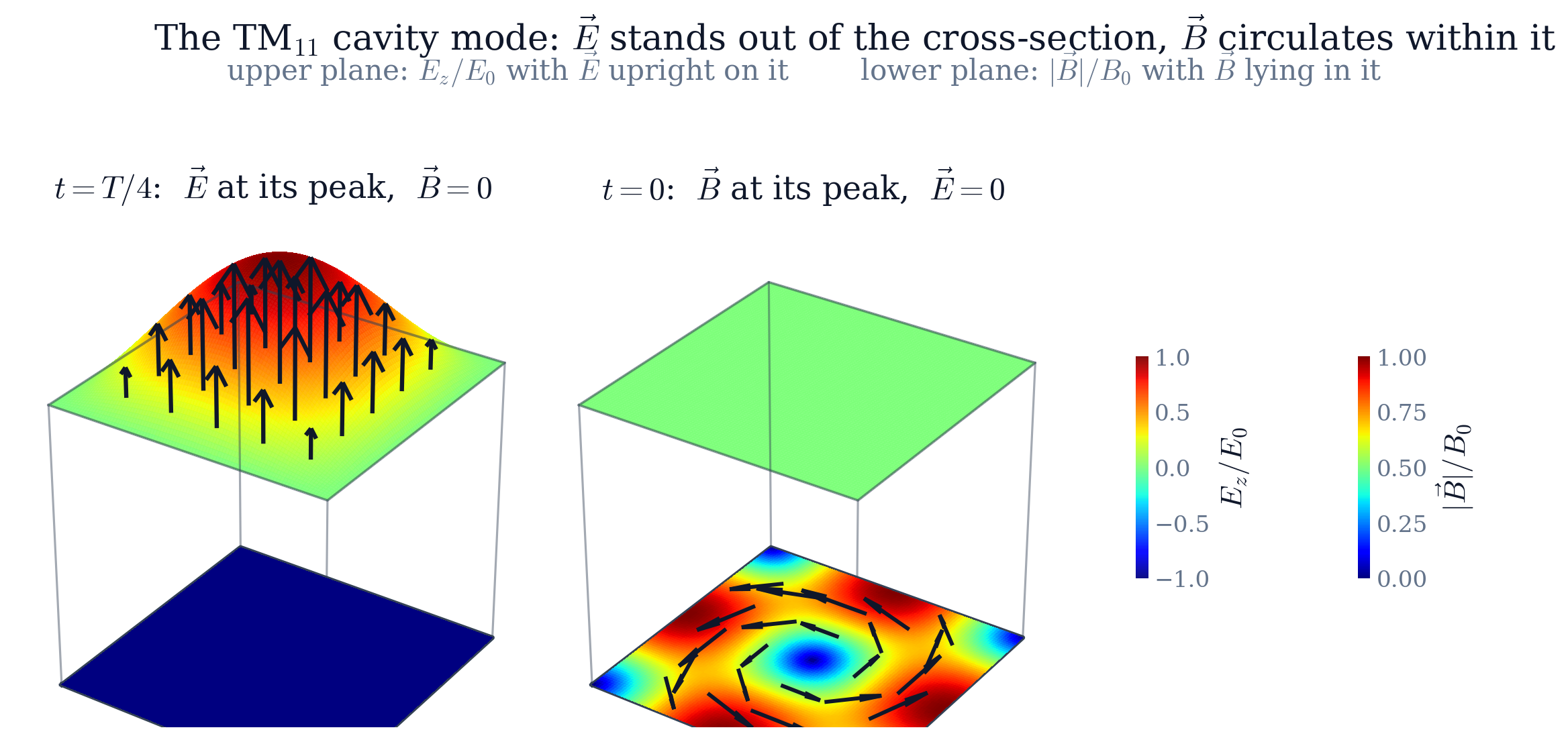
The TM11 cavity mode, drawn twice: at t = T/4, when E is at its peak and B has vanished, and at t = 0, when the reverse holds. In each panel the upper coloured surface is Ez/E0 over the cross-section, with the upright arrows showing E itself running from the plane up to that surface; the lower plane carries |B|/B0 on the same colour map, with arrows giving its direction. Ez is largest at the centre and vanishes on all four walls, as the conducting boundary requires, while B vanishes at the centre and is largest at the wall midpoints — the two fields are out of step in space as well as in time. That neither panel is busy in both halves at once is the quarter-period phase shift, seen directly. — Figure 1. The TM $_{11}$ cavity mode, drawn twice: at $$t = T/4$$ , when $\vec{E}$ is at its peak and $\vec{B}$ has vanished, and at $$t = 0$$ , when the reverse holds. In each panel the upper coloured surface is $$E_z/E_0$$ over the cross-section, with the upright arrows showing $\vec{E}$ itself running from the plane up to that surface; the lower plane carries $|\vec{B}|/B_0$ on the same colour map, with arrows giving its direction. $$E_z$$ is largest at the centre and vanishes on all four walls, as the conducting boundary requires, while $\vec{B}$ vanishes at the centre and is largest at the wall midpoints — the two fields are out of step in space as well as in time. That neither panel is busy in both halves at once is the quarter-period phase shift, seen directly.

Figure 2 runs one full period of the oscillation. Plotting $$E_z$$ as a height turns the standing wave into a surface that swells, flattens and inverts without its shape ever changing; the upright arrows are the electric field vector itself, and $\vec{B}$ — which lies in the plane — is drawn as arrows on the floor beneath. The quarter-period phase shift then needs no explaining: the surface is flat, and the upright arrows are gone, exactly when the floor arrows are longest.

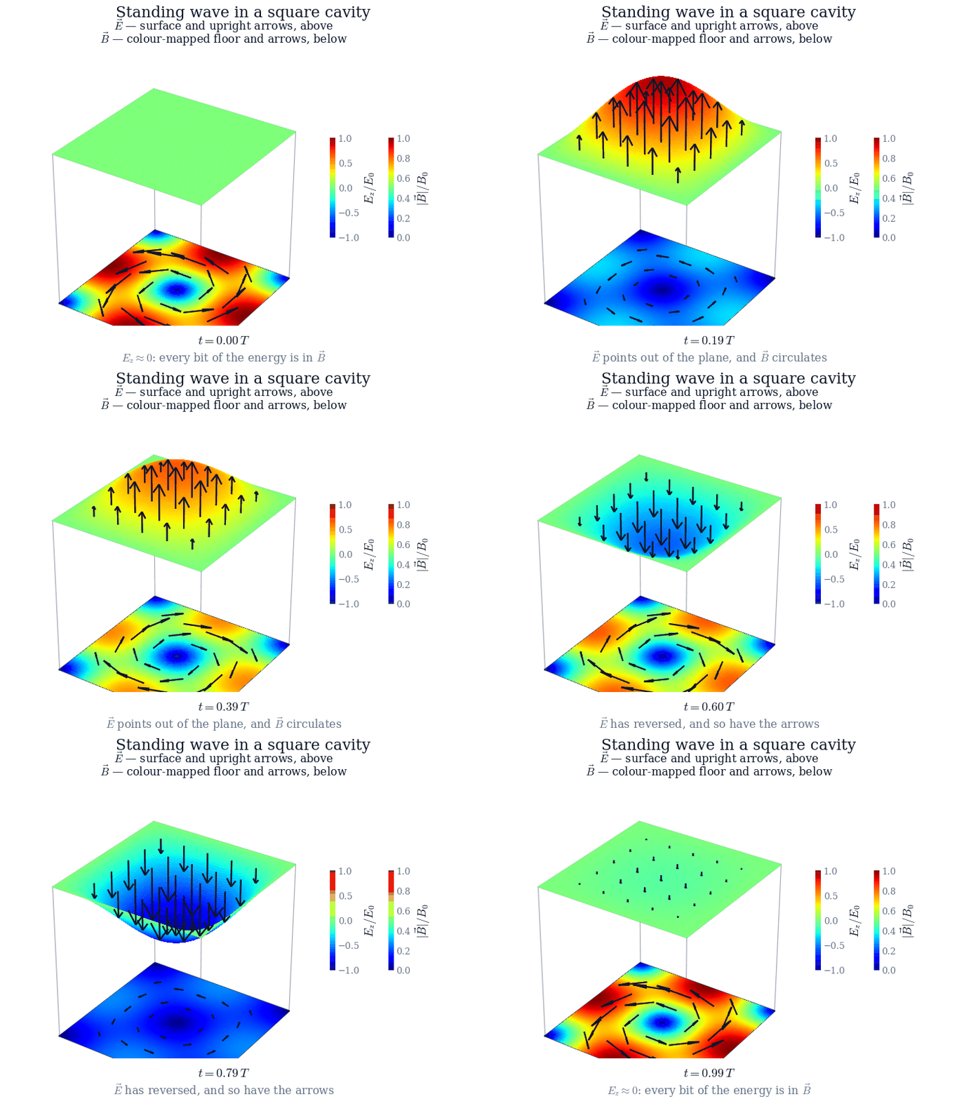
One period of the cavity oscillation. Above: the coloured surface is Ez/E0 and the upright arrows are E. Below: the floor carries |B|/B0 on the same colour map, with arrows for its direction. At t=0 the surface is flat while the floor is at full colour; a quarter period later the surface has swelled to its maximum and the floor has drained to zero; at t=T/2 the surface is flat again and the floor arrows have reversed; at t=3T/4 the whole surface has inverted. The two colour scales differ because Ez is signed and |B| is not. The shape never changes — only its amplitude — which is what makes this a standing wave rather than a travelling one. — Figure 2. One period of the cavity oscillation. Above: the coloured surface is $$E_z/E_0$$ and the upright arrows are $\vec{E}$ . Below: the floor carries $|\vec{B}|/B_0$ on the same colour map, with arrows for its direction. At $$t=0$$ the surface is flat while the floor is at full colour; a quarter period later the surface has swelled to its maximum and the floor has drained to zero; at $$t=T/2$$ the surface is flat again and the floor arrows have reversed; at $$t=3T/4$$ the whole surface has inverted. The two colour scales differ because $$E_z$$ is signed and $|\vec{B}|$ is not. The shape never changes — only its amplitude — which is what makes this a standing wave rather than a travelling one.

5The full family of modes

Nothing above required the particular pattern in $\eqref{eq:Egiven}$ . Solving the cavity from scratch produces every mode it supports, and the given field turns out to be the lowest one.

5.1Wave equation

Take the curl of Faraday's law and use $\nabla \times (\nabla \times \vec{E}) = \nabla(\nabla \cdot \vec{E}) - \nabla^2\vec{E}$ together with $\nabla\cdot\vec{E} = 0$ :

\begin{equation} \nabla^2 \vec{E} = \frac{1}{c^2}\,\frac{\partial ^2 \vec{E}}{\partial t^2}, \qquad\text{and likewise}\qquad \nabla^2 \vec{B} = \frac{1}{c^2}\,\frac{\partial ^2 \vec{B}}{\partial t^2}. \label{eq:wave} \end{equation}

Every Cartesian component of both fields satisfies the same scalar wave equation — the partial differential equation of Chapter 10.

5.2Separation of variables (Chapter 10)

This is the method of Chapter 10 applied unchanged. Look for a solution of $\eqref{eq:wave}$ with no $$z$$ -dependence in the product form $E_z(x,y,t) = X(x)\,Y(y)\,T(t)$ . Substituting and dividing by $$XYT$$ gives

\begin{equation} \frac{X''}{X} + \frac{Y''}{Y} = \frac{1}{c^2}\frac{T''}{T}, \label{eq:separated} \end{equation}

in which the first term depends only on $$x$$ , the second only on $$y$$ and the third only on $$t$$ . Three functions of independent variables can agree only if each is a constant, so $\eqref{eq:separated}$ splits into

\begin{equation} X'' = -k_x^2 X, \qquad Y'' = -k_y^2 Y, \qquad T'' = -\omega^2 T, \qquad \omega^2 = c^2\,(k_x^2 + k_y^2). \label{eq:three-odes} \end{equation}

The signs in $\eqref{eq:three-odes}$ are forced: a positive separation constant would give growing exponentials, which cannot vanish on both walls.

5.3Applying the walls

$$E_z$$ is tangential to all four walls, so it must vanish at $x = \pm L/2$ and at $y = \pm L/2$ . Measuring from the wall at $$x = -L/2$$ , the admissible solutions are

\begin{equation} E_z^{(m,n)}(x,y,t) = E_0 \sin\!\left( \frac{m\pi (x + L/2)}{L} \right) \sin\!\left( \frac{n\pi (y + L/2)}{L} \right) \sin(\omega_{mn} t), \qquad m, n = 1, 2, 3, \dots \label{eq:modes} \end{equation}

with

\begin{equation} \boxed{\;\omega_{mn} = \frac{\pi c}{L}\sqrt{m^2 + n^2}\;} \label{eq:omega-mn} \end{equation}

For $$m = n = 1$$ the shifted sine is just $\cos(\pi x/L)$ , so $\eqref{eq:modes}$ reproduces the field of the problem and $\eqref{eq:omega-mn}$ reproduces $\omega_{11} = \sqrt{2}\pi c/L$ , confirming $\eqref{eq:answer-a}$ . Writing the modes as shifted sines rather than as $\cos(m\pi x/L)$ matters for the higher ones: the plain cosine satisfies the boundary condition only when $$m$$ is odd, and would put an antinode on the conductor when $$m$$ is even.

The six lowest modes are shown in Figure 3. Their frequencies are not multiples of one another — $\sqrt{m^2+n^2}$ is rarely a rational multiple of $\sqrt2$ — and modes related by swapping $$m$$ and $$n$$ are degenerate, sharing one frequency between two distinct field patterns.

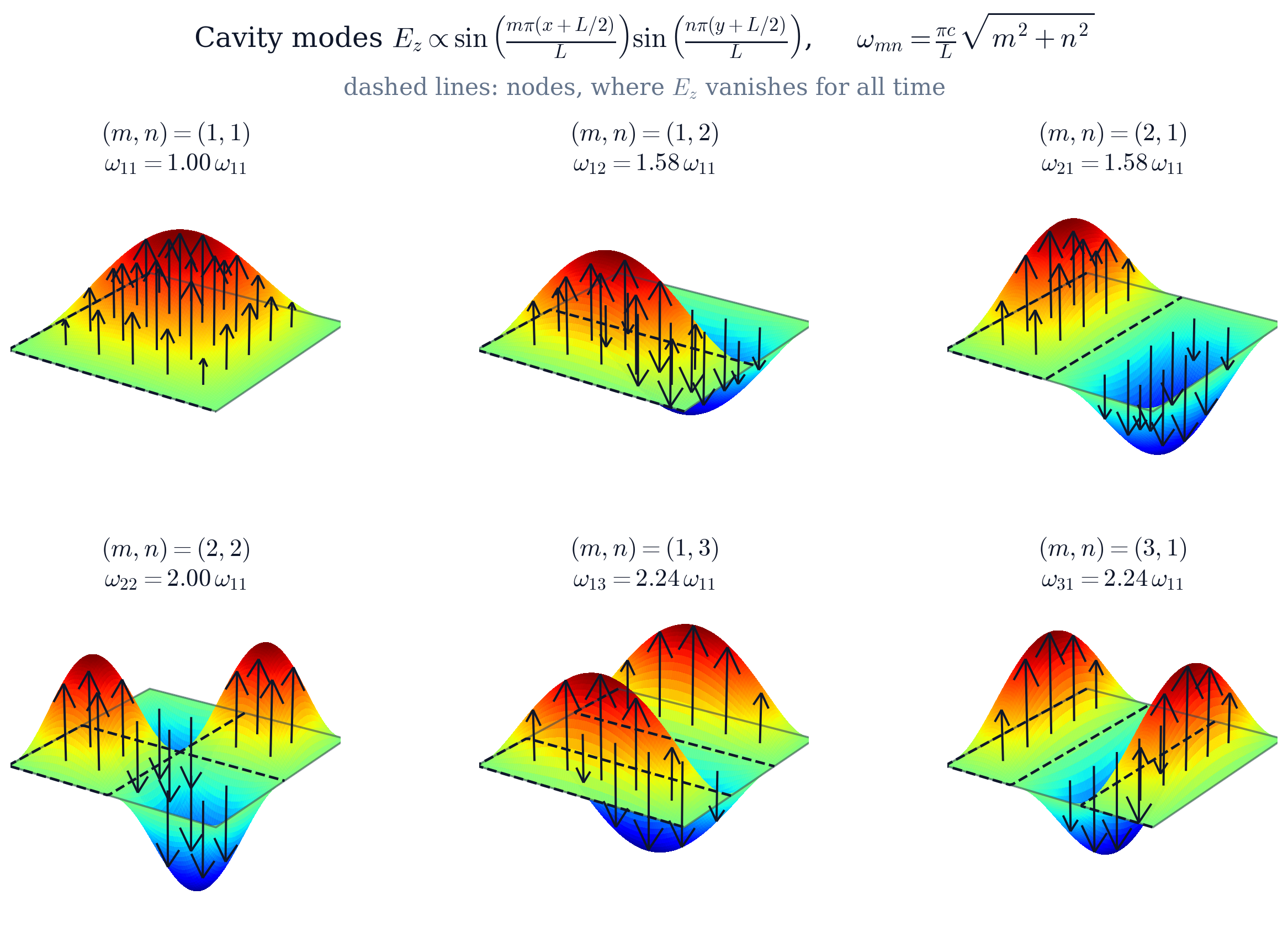
The six lowest cavity modes, each shown as the surface Ez over the cross-section with the field vectors standing on it, and with their frequencies in units of 11. Dashed lines mark the nodes, where Ez is permanently zero and the arrows have no length; on either side of a node the arrows point in opposite directions, which is what a change of sign means physically. The pairs (1,2)/(2,1) and (1,3)/(3,1) are degenerate: the same frequency carried by two different patterns, one the other rotated by a quarter turn. — Figure 3. The six lowest cavity modes, each shown as the surface $$E_z$$ over the cross-section with the field vectors standing on it, and with their frequencies in units of $\omega_{11}$ . Dashed lines mark the nodes, where $$E_z$$ is permanently zero and the arrows have no length; on either side of a node the arrows point in opposite directions, which is what a change of sign means physically. The pairs $$(1,2)$$ / $$(2,1)$$ and $$(1,3)$$ / $$(3,1)$$ are degenerate: the same frequency carried by two different patterns, one the other rotated by a quarter turn.

Once $$E_z$$ is known, $\vec{B}$ follows from Faraday's law, so $\eqref{eq:modes}$ determines the mode completely.

6Energy in the cavity

The energy density of the field is $u = \tfrac{1}{2}\varepsilon_0 E^2 + B^2/(2\mu_0)$ . Integrating it over the cross-section is a double integral of the kind set up in Chapter 5, and the only fact needed is $\int_{-L/2}^{L/2}\cos^2(\pi x/L)\,dx = L/2$ . Using $\eqref{eq:Egiven}$ and $\eqref{eq:Bgiven}$ with $B_0 = E_0/(\sqrt{2}c)$ from $\eqref{eq:answer-a}$ ,

\begin{equation} U_E(t) = \frac{\varepsilon_0 E_0^2 L^2}{8}\,\sin^2(\omega t), \qquad U_B(t) = \frac{\varepsilon_0 E_0^2 L^2}{8}\,\cos^2(\omega t), \end{equation}

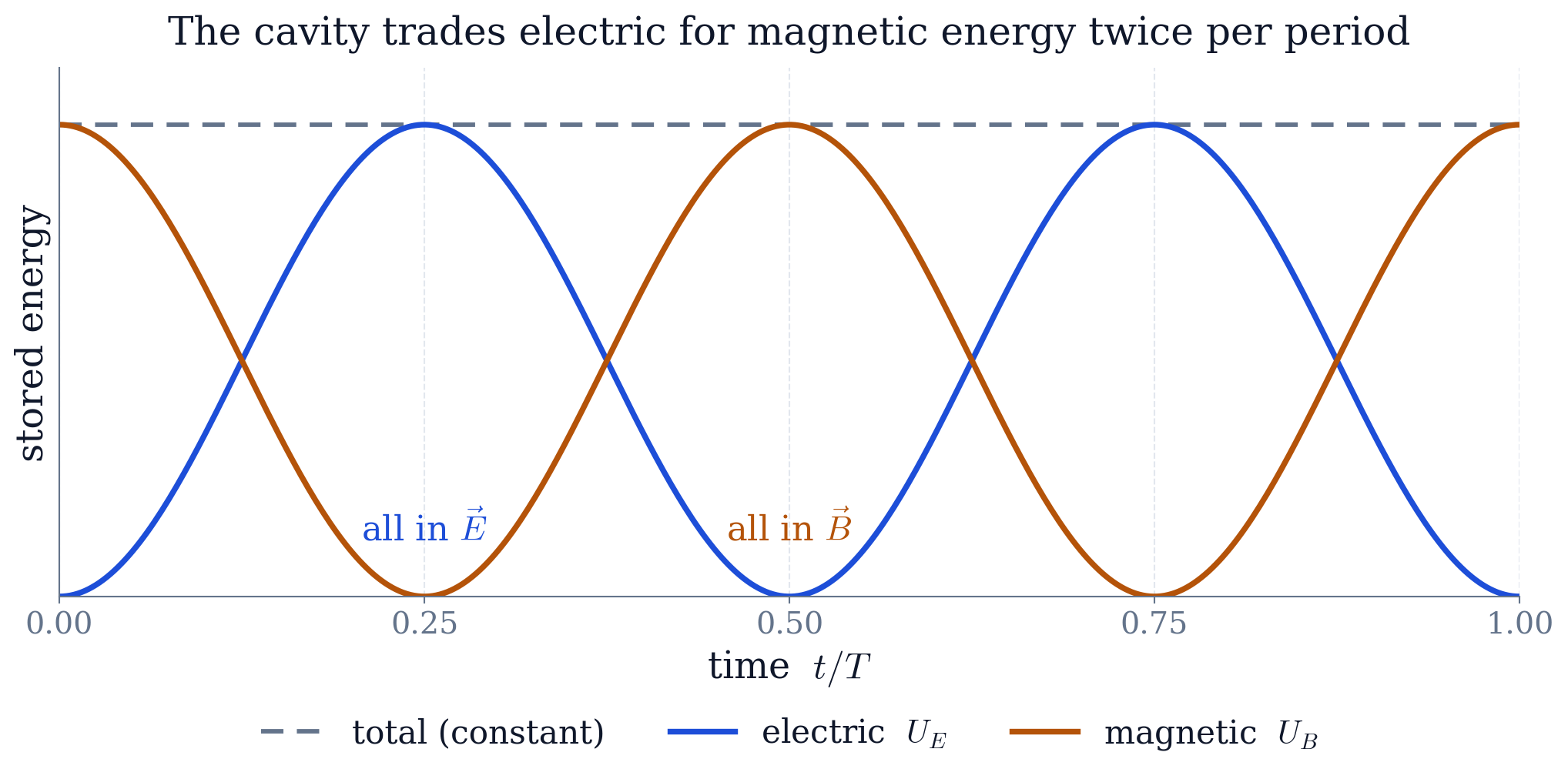
so the total $$U_E + U_B$$ is constant, as it must be for a lossless cavity. The two peak values come out equal — a check the script prints when it runs, and the content of Figure 4. The energy sloshes back and forth between the electric and magnetic field twice per period, exactly as it does between the capacitor and the inductor of an $$LC$$ circuit.

Figure 4. Electric and magnetic energy over one period. Each is largest when the other vanishes, and their sum is constant.

7Which course methods were used

Partial differentiation and vector operators (Chapter 6). Verifying the field is four exercises in taking divergences and curls of products of sines and cosines; the two matching conditions $\eqref{eq:match1}$ – $\eqref{eq:match2}$ fall straight out of them.
Partial differential equations (Chapter 10). Eliminating $\vec{B}$ turns Maxwell's equations into the wave equation, and separation of variables plus the wall conditions turns that into the discrete family $\eqref{eq:modes}$ . The quantisation of $\omega_{mn}$ is a boundary-value problem, not a property of the wave equation itself.
Fourier series (Chapter 7). The modes $\eqref{eq:modes}$ are a complete orthogonal set on the square, so any field the cavity can hold is a double Fourier sine series in these patterns — which is what lets us treat the lowest mode on its own.
Multiple integrals (Chapter 5). The stored energies $$U_E$$ and $$U_B$$ are area integrals of the energy density over the cross-section.

8Conclusion

Requiring the proposed field to satisfy Maxwell's equations in vacuum forces $\omega = \sqrt{2}\pi c/L$ and $B_0 = E_0/(\sqrt{2}c)$ , and the field is then the lowest TM mode of a square cavity. Solving the same problem by separation of variables gives the whole spectrum $\omega_{mn} = (\pi c/L)\sqrt{m^2+n^2}$ , with degenerate pairs whenever $m \neq n$ . The visualisation shows what the algebra states: a field frozen in shape, oscillating in amplitude, passing its energy back and forth between $\vec{E}$ and $\vec{B}$ twice each period, and going to zero at the conducting walls.

References

M. L. Boas, Mathematical Methods in the Physical Sciences, Wiley, 3rd ed., 2006 (Problem 11.13, Chapter 6).
D. J. Griffiths, Introduction to Electrodynamics, Cambridge University Press, 5th ed., 2023 (waveguides and cavities).

← All projects