Chapter 9

Series Solutions of Ordinary Differential Equations (Chapter 12)

9.1Ordinary, Regular Singular, and Irregular Points

Consider the second–order linear differential equation

\begin{equation} y'' + P(x)\,y' + Q(x)\,y = 0, \end{equation}

where \(P(x)\) and \(Q(x)\) are known functions.

Definition - Analytic function

A function \(f(x)\) is called analytic at \(x=x_0\) if it can be written as a convergent power series in a neighborhood of \(x_0\):

\begin{equation} f(x)=\sum_{n=0}^{\infty} c_n(x-x_0)^n. \end{equation}

Analytic functions are finite, smooth, and well behaved near \(x_0\).

Definition

A point \(x=x_0\) of the differential equation is classified as follows:

  • Ordinary point: \(x_0\) is an ordinary point if both \(P(x)\) and \(Q(x)\) are analytic at \(x_0\). All coefficients are finite and smooth, so we may solve the equation using a standard power–series (Taylor) expansion

    \begin{equation} y(x)=\sum_{n=0}^{\infty} A_n (x-x_0)^n. \end{equation}
  • Regular singular point: \(x_0\) is a regular singular point if \(P(x)\) or \(Q(x)\) diverge at \(x_0\), but the combinations

    \begin{equation} (x-x_0)P(x), \qquad (x-x_0)^2 Q(x) \end{equation}

    are analytic at \(x_0\). The singularity is “mild’’ and the correct solution method is the Frobenius method, which assumes

    \begin{equation} y(x)=\sum_{n=0}^{\infty} a_n (x-x_0)^{n+r},\qquad a_0\neq 0. \end{equation}

    This produces an indicial equation for \(r\) and a recurrence for \(a_n\).

  • Irregular singular point: If even \((x-x_0)P(x)\) or \((x-x_0)^2 Q(x)\) fail to be analytic, then the point is an irregular singular point. The singularity is “too strong’’ and ordinary series or Frobenius methods typically fail.

Remark
  • At an ordinary point, use a Taylor series.

  • At a regular singular point, use the Frobenius series.

  • Many special functions in physics—Legendre, Bessel, Hermite, Laguerre—originate from equations with regular singular points, where Frobenius expansions naturally apply.

Example - (ordinary point): Solve \(y' = 2xy\) by two methods

We solve

\begin{equation} y' = 2xy \end{equation}

by (1) the standard separable method and (2) a power–series method about \(x_0=0\).

Method 1: Standard (separable) solution.

For \(y\neq 0\),

\begin{equation} \frac{dy}{dx} = 2xy \quad\Longrightarrow\quad \frac{1}{y}\,dy = 2x\,dx. \end{equation}

Integrate both sides:

\begin{equation} \int \frac{1}{y}\,dy = \int 2x\,dx \quad\Longrightarrow\quad \ln|y| = x^{2} + C. \end{equation}

Exponentiate:

\begin{equation} |y| = e^{x^{2}+C} = e^C e^{x^{2}}. \end{equation}

Let \(C_1 = \pm e^C\) (an arbitrary constant), then

\begin{equation} y(x) = C_1 e^{x^{2}}. \end{equation}

Allowing \(C_1=0\) also includes the trivial solution \(y\equiv 0\):

\begin{equation} \boxed{\,y(x) = C_1 e^{x^{2}},\quad C_1\in\mathbb{R}.\,} \end{equation}

Method 2: Power–series solution about \(x_0=0\).

Assume a power series

\begin{equation} y(x) = \sum_{n=0}^{\infty} a_n x^{n}, \end{equation}

so

\begin{equation} y'(x) = \sum_{n=1}^{\infty} n a_n x^{n-1}. \end{equation}

Substitute into \(y' = 2xy\):

\begin{equation} \sum_{n=1}^{\infty} n a_n x^{n-1} = 2x \sum_{n=0}^{\infty} a_n x^{n} = 2\sum_{n=0}^{\infty} a_n x^{n+1}. \end{equation}

Align the powers of \(x\).

On the left, set \(m=n-1\):

\begin{equation} \sum_{m=0}^{\infty} (m+1)a_{m+1} x^{m}. \end{equation}

On the right, write the sum with index \(m\):

\begin{equation} 2\sum_{m=1}^{\infty} a_{m-1} x^{m}. \end{equation}

Thus

\begin{equation} \sum_{m=0}^{\infty} (m+1)a_{m+1} x^{m} = 2\sum_{m=1}^{\infty} a_{m-1} x^{m}. \end{equation}

For \(m=0\), only the left sum contributes:

\begin{equation} (0+1)a_1 = 0 \quad\Longrightarrow\quad a_1 = 0. \end{equation}

For \(m\ge 1\), equate coefficients of \(x^{m}\):

\begin{equation} (m+1)a_{m+1} = 2a_{m-1}, \qquad m\ge1. \end{equation}

So the recurrence is

\begin{equation} \boxed{\; a_{m+1} = \frac{2}{m+1}\,a_{m-1}, \quad m\ge1. \;} \end{equation}

Compute the coefficients.

\begin{equation} \begin{aligned} m=1:&\quad 2a_2 = 2a_0 \Rightarrow a_2 = a_0,\\ m=2:&\quad 3a_3 = 2a_1 = 0 \Rightarrow a_3 = 0,\\ m=3:&\quad 4a_4 = 2a_2 = 2a_0 \Rightarrow a_4 = \frac{a_0}{2!},\\ m=5:&\quad 6a_6 = 2a_4 = a_0 \Rightarrow a_6 = \frac{a_0}{3!},\ \ldots \end{aligned} \end{equation}

We see

\begin{equation} a_{2k} = \frac{a_0}{k!},\qquad a_{2k+1}=0,\quad k=0,1,2,\ldots \end{equation}

Therefore

\begin{equation} y(x) = a_0\left(1 + x^{2} + \frac{x^{4}}{2!} + \frac{x^{6}}{3!} + \cdots\right) = a_0\sum_{k=0}^{\infty} \frac{x^{2k}}{k!} = a_0 e^{x^{2}}. \end{equation}

Renaming \(a_0\) as \(C_1\), we obtain the same family of solutions:

\begin{equation} \boxed{\,y(x) = C_1 e^{x^{2}},\quad C_1\in\mathbb{R}.\,} \end{equation}

9.2Legendre’s Differential Equation

Many physical systems with spherical symmetry—electrostatics, gravitational potentials, quantum mechanics, and classical wave equations—lead to the Legendre differential equation:

\begin{equation} \boxed{ (1-x^{2})\,y'' - 2x\,y' + \ell(\ell+1)\,y = 0, } \qquad \ell = 0,1,2,\ldots \end{equation}
Remark

The points \(x=\pm1\) are regular singular points, while \(x=0\) is an ordinary point. Therefore ordinary power series work at the center, and Frobenius-type behavior appears at the endpoints.

9.2.1Power–Series Solution About \(x=0\) (Ordinary Point)

We now derive the recurrence relation for the coefficients \(a_n\).

Assume a power–series solution about the ordinary point \(x=0\):

\begin{equation} y(x) = \sum_{n=0}^{\infty} a_n x^n. \end{equation}

Then

\begin{equation} y'(x) = \sum_{n=1}^{\infty} n a_n x^{n-1}, \qquad y''(x) = \sum_{n=2}^{\infty} n(n-1) a_n x^{n-2}. \end{equation}

Substitute these into Legendre’s equation

\begin{equation} (1-x^2)y'' - 2x\,y' + \ell(\ell+1)y = 0: \end{equation}
\begin{equation} (1-x^2)\sum_{n=2}^{\infty} n(n-1)a_n x^{n-2} - 2x \sum_{n=1}^{\infty} n a_n x^{n-1} + \ell(\ell+1)\sum_{n=0}^{\infty} a_n x^n = 0. \end{equation}

First expand the product \((1-x^2)y''\):

\begin{equation} (1-x^2)y'' = \sum_{n=2}^{\infty} n(n-1)a_n x^{n-2} - \sum_{n=2}^{\infty} n(n-1)a_n x^{n}. \end{equation}

Now shift indices so that every sum is in powers of \(x^n\).

For the first sum, let \(k=n-2\) (equivalently \(n=k+2\)):

\begin{equation} \sum_{n=2}^{\infty} n(n-1)a_n x^{n-2} = \sum_{k=0}^{\infty} (k+2)(k+1)a_{k+2} x^{k}. \end{equation}

Renaming \(k\) back to \(n\),

\begin{equation} \sum_{n=0}^{\infty} (n+2)(n+1)a_{n+2} x^{n}. \end{equation}

The other sums already have powers \(x^n\) (we can extend the lower limit to \(0\), since the missing terms are zero):

\begin{equation} - \sum_{n=2}^{\infty} n(n-1)a_n x^{n} = -\sum_{n=0}^{\infty} n(n-1)a_n x^n, \end{equation}
\begin{equation} - 2x \sum_{n=1}^{\infty} n a_n x^{n-1} = -2 \sum_{n=1}^{\infty} n a_n x^{n} = -2\sum_{n=0}^{\infty} n a_n x^n, \end{equation}
\begin{equation} \ell(\ell+1)\sum_{n=0}^{\infty} a_n x^n = \sum_{n=0}^{\infty} \ell(\ell+1)a_n x^n. \end{equation}

Putting all pieces together:

\begin{equation} \sum_{n=0}^{\infty} (n+2)(n+1)a_{n+2} x^{n} - \sum_{n=0}^{\infty} n(n-1)a_{n} x^{n} - 2\sum_{n=0}^{\infty} n a_{n} x^{n} + \sum_{n=0}^{\infty} \ell(\ell+1)a_n x^n = 0. \end{equation}

Combine the last three sums:

\begin{equation} \sum_{n=0}^{\infty} \Big[ (n+2)(n+1)a_{n+2} + \big(\ell(\ell+1) - n(n-1) - 2n\big)a_n \Big] x^n = 0. \end{equation}

Note that

\begin{equation} n(n-1) + 2n = n^2 - n + 2n = n^2 + n = n(n+1), \end{equation}

so

\begin{equation} \ell(\ell+1) - n(n-1) - 2n = \ell(\ell+1) - n(n+1). \end{equation}

Thus

\begin{equation} \sum_{n=0}^{\infty} \Big[ (n+2)(n+1)a_{n+2} + \big(\ell(\ell+1) - n(n+1)\big)a_n \Big] x^n = 0. \end{equation}

For this identity to hold for all \(x\), each coefficient of \(x^n\) must vanish:

\begin{equation} (n+2)(n+1)a_{n+2} + \big(\ell(\ell+1) - n(n+1)\big)a_n = 0. \end{equation}

Solving for \(a_{n+2}\) gives the recurrence

\begin{equation} \boxed{ a_{n+2} = \frac{n(n+1) - \ell(\ell+1)}{(n+1)(n+2)}\,a_n, \qquad n=0,1,2,\ldots } \end{equation}

which determines all higher coefficients from \(a_0\) and \(a_1\). Starting from the recurrence relation

\begin{equation} a_{n+2} = \frac{n(n+1)-\ell(\ell+1)}{(n+1)(n+2)}\,a_n, \qquad n=0,1,2,\ldots, \end{equation}

we compute the first few coefficients.

Coefficient \(a_{2}\).

Set \(n=0\):

\begin{equation} a_{2} = \frac{0\cdot 1 - \ell(\ell+1)}{1\cdot 2}\,a_{0} = -\frac{\ell(\ell+1)}{2}\,a_{0}. \end{equation}

Coefficient \(a_{3}\).

Set \(n=1\):

\begin{equation} a_{3} = \frac{1\cdot 2 - \ell(\ell+1)}{2\cdot 3}\,a_{1} = \frac{2-\ell(\ell+1)}{6}\,a_{1} = -\frac{\ell(\ell+1)-2}{3!}\,a_{1} = -\frac{(\ell-1)(\ell+2)}{3!}\,a_{1}. \end{equation}

Coefficient \(a_{4}\).

Set \(n=2\):

\begin{equation} a_{4} = \frac{2\cdot 3 - \ell(\ell+1)}{3\cdot 4}\,a_{2} = \frac{6-\ell(\ell+1)}{12}\,a_{2}. \end{equation}

Using \(a_{2}=-\dfrac{\ell(\ell+1)}{2}a_{0}\):

\begin{equation} a_{4} = \frac{6-\ell(\ell+1)}{12} \left(-\frac{\ell(\ell+1)}{2}a_{0}\right) = -\frac{\ell(\ell+1)\bigl(6-\ell(\ell+1)\bigr)}{24}\,a_{0}. \end{equation}

Since \(6-\ell(\ell+1)=-(\ell-2)(\ell+3)\), this becomes

\begin{equation} a_{4} = \frac{\ell(\ell+1)(\ell-2)(\ell+3)}{4!}\,a_{0}. \end{equation}

Coefficient \(a_{5}\).

Set \(n=3\):

\begin{equation} a_{5} = \frac{3\cdot 4 - \ell(\ell+1)}{4\cdot 5}\,a_{3} = \frac{12-\ell(\ell+1)}{20}\,a_{3}. \end{equation}

Using \(a_{3}=\dfrac{2-\ell(\ell+1)}{6}a_{1}\):

\begin{equation} a_{5} = \frac{12-\ell(\ell+1)}{20} \cdot \frac{2-\ell(\ell+1)}{6}a_{1} = \frac{(12-\ell(\ell+1))(2-\ell(\ell+1))}{120}\,a_{1}. \end{equation}

Factoring,

\begin{equation} (12-\ell(\ell+1))(2-\ell(\ell+1)) = (\ell-1)(\ell+2)(\ell-3)(\ell+4), \end{equation}

so

\begin{equation} a_{5} = \frac{(\ell-1)(\ell+2)(\ell-3)(\ell+4)}{5!}\,a_{1}. \end{equation}

Therefore

\begin{equation} \boxed{ \begin{aligned} a_{2} &= -\dfrac{\ell(\ell+1)}{2}\,a_{0},\\[6pt] a_{3} &= -\frac{(\ell-1)(\ell+2)}{3!}\,a_{1},\\[6pt] a_{4} &= \dfrac{\ell(\ell+1)(\ell-2)(\ell+3)}{4!}\,a_{0},\\[6pt] a_{5} &= \dfrac{(\ell-1)(\ell+2)(\ell-3)(\ell+4)}{5!}\,a_{1}. \end{aligned} } \end{equation}
Remark

Even coefficients depend only on \(a_0\); odd coefficients depend only on \(a_1\). Thus the general solution splits into two independent series: one even in \(x\), built from \(a_0\), and one odd in \(x\), built from \(a_1\).

\begin{equation} \begin{aligned} y(x)=\sum_{n=0}^{\infty} a_n x^n = &\; a_{0}\Bigl[ 1 - \frac{\ell(\ell+1)}{2!}x^{2} + \frac{\ell(\ell+1)(\ell-2)(\ell+3)}{4!}x^{4} - \cdots \Bigr] \\[6pt] &\quad + a_{1}\Bigl[ x - \frac{(\ell-1)(\ell+2)}{3!}x^{3} + \frac{(\ell-1)(\ell+2)(\ell-3)(\ell+4)}{5!}x^{5} - \cdots \Bigr]. \end{aligned} \end{equation}

9.2.2Polynomial Solutions: the Legendre Polynomials

Now restrict to the physically important case where \(\ell\) is a non-negative integer. The recurrence factor

\begin{equation} n(n+1)-\ell(\ell+1) \end{equation}

vanishes when \(n=\ell\). Since even coefficients use \(n=0,2,4,\dots\) and odd coefficients use \(n=1,3,5,\dots\), the vanishing occurs either in the even or odd subsequence:

Thus for each integer \(\ell\), exactly one of the two series becomes a finite polynomial of degree \(\ell\). This terminating series, normalized by \(P_\ell(1)=1\), is the Legendre polynomial \(P_\ell(x)\).

We now illustrate this for \(\ell=0,1,2,3,4\), always normalizing with \(P_\ell(1)=1\).

Case \(\ell = 0\)

Here \(\ell(\ell+1)=0\). The even series gives

\begin{equation} a_0\bigl[\,1-0\cdot x^2+0\cdot x^4-\cdots\,\bigr]=a_0. \end{equation}

The odd series does not terminate. To obtain the polynomial solution, choose \(a_0\neq 0\) and set \(a_1=0\). Normalization \(P_0(1)=1\) gives \(a_0=1\), hence

\begin{equation} \boxed{P_{0}(x)=1.} \end{equation}

Case \(\ell = 1\)

Here \(\ell(\ell+1)=2\). The odd series is

\begin{equation} a_1\left[ x - \frac{2-2}{3!}x^{3} + \cdots \right] = a_1 x, \end{equation}

since the coefficient of \(x^3\) vanishes. The even series does not terminate. To get the polynomial, choose \(a_1\neq 0\), \(a_0=0\). With \(P_1(1)=1\), we take \(a_1=1\) and obtain

\begin{equation} \boxed{P_{1}(x)=x.} \end{equation}

Case \(\ell = 2\)

Here \(\ell(\ell+1)=6\). The even series begins

\begin{equation} a_0\left[ 1 - \frac{6}{2!} x^{2} + \cdots \right] = a_0\left[1 - 3x^2 + \cdots\right]. \end{equation}

At \(n=2\), the factor \(n(n+1)-\ell(\ell+1)=6-6=0\), so \(a_4\) and all higher even coefficients vanish and the even series terminates at \(x^2\):

\begin{equation} a_0\left(1 - 3x^2\right). \end{equation}

The odd series does not terminate. Choose \(a_0\neq 0,\;a_1=0\) and normalize with \(P_2(1)=1\). Since the polynomial at \(x=1\) is \(a_0(1-3)=-2a_0\),

\begin{equation} -2a_0 = 1 \quad\Rightarrow\quad a_0=-\tfrac12, \end{equation}

so

\begin{equation} \boxed{P_2(x)=-\tfrac12\left(1 - 3x^2\right)=\tfrac12(3x^2-1).} \end{equation}

Case \(\ell = 3\)

Here \(\ell(\ell+1)=12\). The odd series is

\begin{equation} a_1\left[ x - \frac{12-2}{3!}x^{3} + \cdots \right] = a_1\left[x - \frac{10}{6}x^3 + \cdots\right] = a_1\left[x - \frac{5}{3}x^3 + \cdots\right]. \end{equation}

At \(n=3\), the factor \(n(n+1)-\ell(\ell+1)=12-12=0\), so higher odd coefficients vanish and the odd series terminates at \(x^3\):

\begin{equation} a_1\left(x - \tfrac{5}{3}x^3\right). \end{equation}

The even series does not terminate. To obtain the polynomial, choose \(a_1\neq 0,\;a_0=0\) and normalize with \(P_3(1)=1\). Since the polynomial at \(x=1\) is \(a_1(1-\tfrac53)=-\tfrac23 a_1\),

\begin{equation} -\tfrac23 a_1 = 1 \quad\Rightarrow\quad a_1=-\tfrac32, \end{equation}

so

\begin{equation} \boxed{P_3(x)=-\tfrac32\left(x - \tfrac{5}{3}x^3\right)=\tfrac12(5x^3-3x).} \end{equation}

Case \(\ell = 4\)

Here \(\ell(\ell+1)=20\). The even series is

\begin{equation} a_0\left[ 1 - \frac{20}{2!}x^{2} + \frac{20(2)(7)}{4!}x^{4} - \cdots \right] = a_0\left[1 - 10x^2 + \frac{35}{3}x^4 - \cdots\right]. \end{equation}

At \(n=4\), the factor \(n(n+1)-\ell(\ell+1)=20-20=0\), so higher even coefficients vanish and the even series terminates. The odd series does not terminate. Choose \(a_0\neq 0,\;a_1=0\) and normalize with \(P_4(1)=1\):

\begin{equation} a_0=\frac{3}{8}, \end{equation}

giving

\begin{equation} \boxed{P_4(x)=\tfrac18(35x^4-30x^2+3).} \end{equation}

Therefore Legendre Polynomials are

\begin{equation} \begin{aligned} P_0(x) &= 1,\\[4pt] P_1(x) &= x,\\[4pt] P_2(x) &= \tfrac12(3x^2 - 1),\\[4pt] P_3(x) &= \tfrac12(5x^3 - 3x),\\[4pt] P_4(x) &= \tfrac18(35x^4 - 30x^2 + 3),\;\ldots \end{aligned} \end{equation}

These polynomials appear throughout physics, especially in problems involving spherical symmetry such as multipole expansions, potential theory, and quantum angular momentum.

Radius of Convergence and Interval of Validity

For large \(n\),

\begin{equation} \frac{n(n+1)-\ell(\ell+1)}{(n+1)(n+2)} \sim \frac{n^2}{n^2} =1. \end{equation}

Thus from

\begin{equation} a_{n+2} = \frac{n(n+1)-\ell(\ell+1)}{(n+1)(n+2)}\,a_n. \end{equation}

we get

\begin{equation} a_{n+2}\sim a_n, \qquad\text{for } n\gg 1. \end{equation}

This means that the coefficients behave like those of the geometric series

\begin{equation} 1 + x^2 + x^4 + \cdots \quad\text{or}\quad x + x^3 + x^5 + \cdots, \end{equation}

both of which converge only when \(|x|<1\).

This immediately gives

\begin{equation} \boxed{R = 1 \quad \text{(radius of convergence).}} \end{equation}

Behavior at the endpoints.

At \(x=\pm1\), the general term behaves like

\begin{equation} a_{2n}(\pm1)^{2n} \sim a_{2n}, \qquad a_{2n+1}(\pm1)^{2n+1} \sim a_{2n+1}, \end{equation}

and since

\begin{equation} a_{n+2}\sim a_n, \end{equation}

the terms do not tend to zero rapidly enough to converge. Typical endpoint behavior is of the form

\begin{equation} 1 + \frac{1}{3} + \frac{1}{5} + \cdots, \end{equation}

which diverges. Therefore,

\begin{equation} \boxed{ \text{the series solution diverges at } x=\pm1. } \end{equation}

Only when the series terminates—that is, when \(\ell\) is a nonnegative integer—do we obtain a polynomial that is finite at the endpoints.

Interval of validity.

For non-terminating solutions,

\begin{equation} y(x)=\sum_{n=0}^\infty a_n x^n \quad \text{is valid only for}\quad -1 < x < 1. \end{equation}

For terminating solutions (the Legendre polynomials \(P_\ell(x)\)), the result is a finite polynomial of degree \(\ell\), so

\begin{equation} \boxed{ P_\ell(x)\ \text{is valid and finite on the entire interval }[-1,1]. } \end{equation}
Remark

In physical applications, \(x=\cos\theta\) ranges over \([-1,1]\). Therefore only the terminating solutions—Legendre polynomials—are acceptable, while the second independent solution diverges at the endpoints.

Rodrigues’ Formula for Legendre Polynomials

Another elegant way of generating these polynomials is provided by Rodrigues’ formula.

Theorem - Rodrigues’ Formula
\begin{equation} \boxed{ P_\ell(x) = \frac{1}{2^\ell \ell!}\,\frac{d^\ell}{dx^\ell}\left( x^2 - 1 \right)^\ell } \end{equation}

This formula expresses the Legendre polynomial \( P_\ell(x) \) as the \(\ell\)-th derivative of the simple algebraic function \( (x^2 - 1)^\ell \). It provides a direct computational method for generating all Legendre polynomials.

9.2.5Examples

Example - 1: Compute \( P_0(x) \) from Rodrigues’ formula

For \( \ell = 0 \):

\begin{equation} (x^2 - 1)^0 = 1, \qquad \frac{d^0}{dx^0}(1) = 1. \end{equation}

Thus,

\begin{equation} P_0(x) = \frac{1}{2^0 0!}\cdot 1 = 1. \end{equation}

P_0(x) = 1

This matches the known result.

Example - 2: Compute \( P_1(x) \) from Rodrigues’ formula

For \( \ell = 1 \):

\begin{equation} (x^2 - 1)^1 = x^2 - 1. \end{equation}

Differentiate once:

\begin{equation} \frac{d}{dx}(x^2 - 1) = 2x. \end{equation}

Now apply Rodrigues’ formula:

\begin{equation} P_1(x) = \frac{1}{2^1 1!}(2x) = x. \end{equation}

P_1(x) = x

Again this matches the standard Legendre polynomial.

Example - 3: Compute \( P_2(x) \) from Rodrigues' formula

For \( \ell = 2 \):

\begin{equation} (x^2-1)^2 = x^4 - 2x^2 + 1. \end{equation}

Differentiate twice:

\begin{equation} \frac{d}{dx}(x^4 - 2x^2 + 1) = 4x^3 - 4x, \end{equation}
\begin{equation} \frac{d^2}{dx^2}(x^4 - 2x^2 + 1) = 12x^2 - 4. \end{equation}

Apply the normalization factor, noting that \(2^2\,2! = 4\cdot 2 = 8\):

\begin{equation} P_2(x) = \frac{1}{2^2\,2!}(12x^2 - 4) = \frac{1}{8}(12x^2 - 4) = \frac{1}{8}\cdot 4(3x^2 - 1) = \frac{1}{2}(3x^2 - 1). \end{equation}

P_2(x) = 12(3x^2 - 1)

Orthogonality

The Legendre polynomials satisfy an essential orthogonality relation on \([-1,1]\):

\begin{equation} \boxed{ \int_{-1}^{1} P_\ell(x)P_m(x)\,dx =\frac{2}{2\ell+1}\,\delta_{\ell m}. } \end{equation}
Remark

Orthogonality makes the Legendre polynomials a natural basis for expanding any sufficiently smooth function on \([-1,1]\). This is the spherical analogue of Fourier series.

Plot of Legendre Polynomials

Figure 9.1 shows the first six Legendre polynomials \(P_0(x)\) through \(P_5(x)\) on the interval \(-1 \le x \le 1\). These polynomials are finite everywhere on the interval, alternate between even and odd parity, and exhibit an increasing number of oscillations with order.

The Legendre polynomials P0(x)–P5(x) plotted on [-1,1].
Figure 9.1. The Legendre polynomials \(P_0(x)\)\(P_5(x)\) plotted on \([-1,1]\).

9.2.8Generating Function

The Legendre polynomials have a remarkable generating function:

\begin{equation} \boxed{ G(x,t)=\frac{1}{\sqrt{1-2xt+t^2}}=\sum_{\ell=0}^{\infty} P_\ell(x)t^\ell. } \end{equation}

For any power series

\begin{equation} f(t) = \sum_{\ell=0}^{\infty} c_\ell t^\ell, \end{equation}

we can recover the coefficients by

\begin{equation} c_\ell = \frac{1}{\ell!}\, \frac{d^\ell f}{dt^\ell}\Big|_{t=0}. \end{equation}

Here, \(x\) is treated as a constant parameter and \(t\) is the series variable. Applying this to the generating function,

\begin{equation} G(x,t) = \sum_{\ell=0}^{\infty} P_\ell(x)\, t^\ell, \end{equation}

we get

\begin{equation} \boxed{ P_\ell(x) = \frac{1}{\ell!}\,\frac{\partial^\ell}{\partial t^\ell} \left[ \frac{1}{\sqrt{1-2xt+t^{2}}} \right]_{t=0}. } \end{equation}
Example - Computing the first few Legendre polynomials from \(G(x,t)\)

(a) \(\ell=0\).

\begin{equation} P_0(x) = G(x,0) = \frac{1}{\sqrt{1-0+0}} = 1. \end{equation}

(b) \(\ell=1\). First derivative:

\begin{equation} \frac{\partial G}{\partial t} = \frac{\partial}{\partial t}(1-2xt+t^{2})^{-1/2} = -\tfrac12(1-2xt+t^{2})^{-3/2}(-2x+2t) = (x - t)(1-2xt+t^{2})^{-3/2}. \end{equation}

Evaluate at \(t=0\):

\begin{equation} P_1(x) = \frac{\partial G}{\partial t}\Big|_{t=0} = x. \end{equation}

(c) \(\ell=2\). Second derivative:

\begin{equation} P_2(x) = \frac{1}{2!}\,\frac{\partial^2 G}{\partial t^2}\Big|_{t=0}. \end{equation}

Carrying out the differentiation (or using a CAS) gives

\begin{equation} P_2(x) = \tfrac12(3x^2 - 1). \end{equation}

(d) \(\ell=3\).

\begin{equation} P_3(x) = \frac{1}{3!}\,\frac{\partial^3 G}{\partial t^3}\Big|_{t=0} = \tfrac12(5x^3 - 3x). \end{equation}

Thus the generating function indeed reproduces the familiar Legendre polynomials:

\begin{equation} P_0(x)=1,\quad P_1(x)=x,\quad P_2(x)=\tfrac12(3x^2-1),\quad P_3(x)=\tfrac12(5x^3-3x),\ \ldots \end{equation}

9.3Associated Legendre Functions

The associated Legendre functions arise naturally when solving Laplace’s equation or the angular part of the Schrödinger equation in spherical coordinates. They generalize the Legendre polynomials by introducing an integer parameter \(m\) that accounts for the dependence on the azimuthal angle \(\phi\).

9.3.1Differential Equation

Starting from separation of variables on the sphere, the angular function \(P_\ell^m(x)\) satisfies the associated Legendre differential equation

\begin{equation} \boxed{ (1-x^2)\,y'' - 2x\,y' + \left[\ell(\ell+1) - \frac{m^2}{1-x^2}\right] y = 0, } \qquad -1 \le x \le 1, \end{equation}

where

\begin{equation} \ell = 0,1,2,\ldots,\qquad m = 0,1,2,\ldots,\ell. \end{equation}

For \(m=0\), the equation reduces to Legendre’s equation.

Remark

The points \(x=\pm1\) are regular singular points. A Frobenius expansion shows that near \(x=\pm1\) the solution behaves as \((1-x^2)^{m/2}\), which guarantees finiteness for integer \(m\).

9.3.2Generating the Solutions

The associated Legendre functions can be obtained from the Legendre polynomials by repeated differentiation:

\begin{equation} \boxed{ P_\ell^{\,m}(x) = (-1)^m(1-x^2)^{m/2}\,\frac{d^m}{dx^m} P_\ell(x). } \end{equation}

This formula produces all associated functions once \(P_\ell(x)\) is known.

Examples:

\begin{equation} \begin{aligned} P_1^1(x) &= -(1-x^2)^{1/2},\\[4pt] P_2^1(x) &= -3x(1-x^2)^{1/2},\\[4pt] P_2^2(x) &= 3(1-x^2). \end{aligned} \end{equation}
Remark

When \(m\) is even, \(P_\ell^m(x)\) has the same parity as \(P_\ell(x)\):

\begin{equation} P_\ell^m(-x)=(-1)^{\ell+m} P_\ell^m(x). \end{equation}

9.3.3Orthogonality

For fixed \(m\), the associated Legendre functions are orthogonal on \([-1,1]\):

\begin{equation} \boxed{ \int_{-1}^{1} P_\ell^m(x)\,P_{\ell'}^m(x)\,dx = \frac{2(\ell+m)!}{(2\ell+1)(\ell-m)!}\,\delta_{\ell\ell'}. } \end{equation}

This extends the orthogonality of Legendre polynomials to functions of higher order \(m\).

Remark

Because of this orthogonality, associated Legendre functions play the same role in spherical problems that sines and cosines play in problems with Cartesian symmetry.

9.3.4Connection to Spherical Harmonics

The full angular dependence of Laplace’s equation and the angular part of the Schrödinger equation in spherical coordinates is expressed using the spherical harmonics:

\begin{equation} \boxed{ Y_{\ell m}(\theta,\phi) = N_{\ell m}\,P_{\ell}^{\,m}(\cos\theta)\,e^{im\phi}, } \qquad \ell = 0,1,2,\ldots, \qquad m = -\ell,\ldots,\ell. \end{equation}

Normalization constant.

The spherical harmonics are orthonormal on the unit sphere,

\begin{equation} \int_{0}^{2\pi}\!\!\int_{0}^{\pi} Y_{\ell m}(\theta,\phi)\,Y_{\ell' m'}^{*}(\theta,\phi)\, \sin\theta\, d\theta\, d\phi =\delta_{\ell\ell'}\delta_{mm'}. \end{equation}

This is achieved when

\begin{equation} \boxed{ N_{\ell m} = (-1)^{m} \sqrt{\frac{2\ell+1}{4\pi}\, \frac{(\ell-m)!}{(\ell+m)!}}. } \end{equation}

The factor \((-1)^{m}\) (the Condon–Shortley phase) is conventional and ensures consistency with standard quantum mechanics notation.

Remark - Physical meaning
  • Each pair \((\ell,m)\) labels an angular momentum eigenstate.

  • \(P_{\ell}^{\,m}(\cos\theta)\) describes the dependence on the polar angle \(\theta\).

  • \(e^{im\phi}\) carries the azimuthal dependence and corresponds to the \(z\)-component of angular momentum.

  • Higher \(|m|\) values push the probability toward the equator (\(\theta=\pi/2\)), reflecting the classical picture of a rotating object with greater projection of angular momentum about the \(z\)-axis.

Thus, the associated Legendre functions provide the essential angular structure of all spherical harmonics.

9.4Bessel’s Differential Equation

Bessel’s equation appears naturally in problems with cylindrical symmetry: heat conduction in cylinders, vibrations of circular membranes (“drumhead problem”), electromagnetic waves in cylindrical waveguides, and quantum mechanics in cylindrical potentials.

The Bessel differential equation of order \(p\) is

\begin{equation} \boxed{ x^{2}y'' + x y' + (x^{2} - p^{2})y = 0, } \qquad p \in \mathbb{R}. \end{equation}
Remark

The point \(x=0\) is a regular singular point. Therefore we must use the Frobenius method (generalized power series). For \(x>0\), all coefficients are analytic and the equation is perfectly regular.

9.4.1Frobenius Series Solution About \(x=0\) (Regular Singular Point)

We seek a generalized power series (Frobenius expansion)

\begin{equation} y(x) = \sum_{n=0}^\infty a_n x^{n+r}, \qquad a_0\neq 0, \end{equation}

where the exponent \(r\) is to be determined.

Compute derivatives:

\begin{equation} y' = \sum_{n=0}^\infty (n+r)a_n x^{n+r-1}, \qquad y'' = \sum_{n=0}^\infty (n+r)(n+r-1)a_n x^{n+r-2}. \end{equation}

Substitute into Bessel’s equation:

\begin{equation} x^2 y'' + x y' + (x^2 - p^2)y = 0. \end{equation}

We obtain:

\begin{equation} x^2 \sum_{n=0}^\infty (n+r)(n+r-1)a_n x^{n+r-2} + x \sum_{n=0}^\infty (n+r)a_n x^{n+r-1} + (x^2 - p^2)\sum_{n=0}^\infty a_n x^{n+r} = 0. \end{equation}

Simplifying each term:

\begin{equation} \sum_{n=0}^\infty (n+r)(n+r-1)a_n x^{n+r} + \sum_{n=0}^\infty (n+r)a_n x^{n+r} + \sum_{n=0}^\infty a_n x^{n+r+2} - p^2\sum_{n=0}^\infty a_n x^{n+r} = 0. \end{equation}

Combine the first three sums:

\begin{equation} (n+r)(n+r-1)+(n+r)-p^2=(n+r)^2-p^2. \end{equation}

Thus,

\begin{equation} \sum_{n=0}^\infty\big[(n+r)^2-p^2\big]a_n x^{n+r} + \sum_{n=0}^\infty a_n x^{n+r+2}=0. \end{equation}

Shift the index in the \(x^{n+r+2}\) term. Starting from

\begin{equation} \sum_{n=0}^{\infty} a_n x^{n+r+2}, \end{equation}

let \(m = n+2\) (so \(n = m-2\)). Then

\begin{equation} \sum_{n=0}^{\infty} a_n x^{n+r+2} = \sum_{m=2}^{\infty} a_{m-2} x^{m+r}. \end{equation}

Renaming the index \(m \to n\) gives

\begin{equation} \sum_{n=0}^\infty\big[(n+r)^2-p^2\big]a_n x^{n+r} + \sum_{n=2}^\infty a_{n-2} x^{n+r}=0. \end{equation}

Now all powers of \(x\) match:

\begin{equation} (r^2 - p^2)\, a_0 x^r + \big[(1+r)^2 - p^2\big] a_1 x^{r+1} + \sum_{n=2}^\infty \Big[ \big((n+r)^2-p^2\big)a_n + a_{n-2} \Big] x^{n+r} = 0. \end{equation}

Because this holds for all \(x\), each coefficient must vanish:

To obtain a solution that stays finite at \(x=0\), we choose the positive root \(r = p\). Then the recurrence becomes

\begin{equation} a_n = -\frac{a_{n-2}}{(n+p)^2 - p^2} = -\frac{a_{n-2}}{n(n+2p)}. \end{equation}

Since \(a_1=0\), all odd coefficients are zero. We therefore write \(n=2k\) (even index) and obtain

\begin{equation} \boxed{ a_{2k} = -\frac{a_{2k-2}}{(2k+p)^2 - p^2} = -\frac{a_{2k-2}}{2k(2k+2p)} = -\frac{a_{2k-2}}{2^{2}k(k+p)}. } \tag{$\star$} \end{equation}

Gamma Function and Coefficient Formula

Definition - Gamma Function

For \(\operatorname{Re}(z)>0\), the Gamma function is defined by

\begin{equation} \Gamma(z) = \int_{0}^{\infty} t^{z-1} e^{-t}\,dt. \end{equation}

It satisfies the recursion

\begin{equation} \Gamma(z+1) = z\,\Gamma(z), \end{equation}

and in particular, for a positive integer \(n\),

\begin{equation} \Gamma(n+1) = n!. \end{equation}

We now use the recurrence \((\star)\) to write the first few even coefficients in a systematic way.

For \(k=1\):

\begin{equation} a_2 = -\frac{a_0}{2^{2}\,1(1+p)} = -\frac{a_0}{2^{2}(1+p)} = -\frac{a_0\,\Gamma(1+p)}{2^{2}\,\Gamma(2+p)}. \end{equation}

For \(k=2\):

\begin{equation} a_4 = -\frac{a_2}{2^{2}\,2(2+p)} = \frac{a_0}{2^{4}\,2!(1+p)(2+p)} = \frac{a_0\,\Gamma(1+p)}{2^{4}\,2!\,\Gamma(3+p)}. \end{equation}

For \(k=3\):

\begin{equation} a_6 = -\frac{a_4}{2^{2}\,3(3+p)} = -\frac{a_0}{2^{6}\,3!(1+p)(2+p)(3+p)} = -\frac{a_0\,\Gamma(1+p)}{2^{6}\,3!\,\Gamma(4+p)}. \end{equation}

We see the pattern: each new \(a_{2k}\) picks up a factor \(-1/[2^{2}k(k+p)]\), which builds up the factorials and Gamma functions.

By induction, the general even coefficient is

\begin{equation} \boxed{ a_{2k} = \frac{(-1)^k\,a_0\,\Gamma(1+p)} {2^{2k}\,k!\,\Gamma(k+1+p)}, \qquad k=0,1,2,\dots } \tag{$\dagger$} \end{equation}

(For \(k=0\) this gives \(a_0\) back.)

Constructing the Series Solution

Our Frobenius ansatz was

\begin{equation} y(x) = \sum_{n=0}^{\infty} a_n x^{n+r}, \qquad r=p. \end{equation}

Since only even \(n\) survive,

\begin{equation} y(x) = \sum_{k=0}^{\infty} a_{2k}\,x^{2k+p}. \end{equation}

Insert the general coefficient (\(\dagger\)):

\begin{equation} \begin{aligned} y(x) &= \sum_{k=0}^{\infty} \frac{(-1)^k\,a_0\,\Gamma(1+p)}{2^{2k}k!\,\Gamma(k+1+p)}\,x^{2k+p} \\[4pt] &= a_0\,\Gamma(1+p)\,x^{p} \sum_{k=0}^{\infty} \frac{(-1)^k}{k!\,\Gamma(k+1+p)} \left(\frac{x^2}{2^{2}}\right)^{k} \\[4pt] &= a_0\,\Gamma(1+p)\, \sum_{k=0}^{\infty} \frac{(-1)^k}{k!\,\Gamma(k+1+p)} \left(\frac{x}{2}\right)^{2k+p}. \end{aligned} \end{equation}

So

\begin{equation} \boxed{ y(x) = a_0\,\Gamma(1+p) \sum_{k=0}^{\infty} \frac{(-1)^k}{k!\,\Gamma(k+p+1)} \left(\frac{x}{2}\right)^{2k+p}. } \end{equation}

To obtain the standard Bessel function of the first kind \(J_p(x)\), we choose \(a_0\) so that the prefactor becomes 1. A convenient choice is

\begin{equation} a_0 = \frac{1}{2^{p}\Gamma(1+p)}. \end{equation}

Then

\begin{equation} a_0\,\Gamma(1+p) = \frac{1}{2^{p}}, \end{equation}

and we arrive at the final series:

\begin{equation} \boxed{ J_p(x) = \sum_{k=0}^{\infty} \frac{(-1)^k}{k!\,\Gamma(k+p+1)} \left(\frac{x}{2}\right)^{2k+p}, } \end{equation}

and the second solution is given by \( J_{-p}(x) \)

The First Solution for Integer Order

For integer order \(p=n\), the general series reduces to

\begin{equation} \boxed{ J_n(x) = \sum_{k=0}^{\infty} \frac{(-1)^k}{k!\,(n+k)!} \left(\frac{x}{2}\right)^{2k+n} } \end{equation}

since \(\Gamma(n+k+1) = (n+k)!\). This is the standard power–series definition of the Bessel function of the first kind. Small-order Bessel functions follow immediately:

\begin{equation} \begin{aligned} J_0(x) &= 1 - \frac{x^{2}}{4} + \frac{x^{4}}{64} - \frac{x^{6}}{2304} + \cdots,\\[6pt] J_1(x) &= \frac{x}{2} - \frac{x^{3}}{16} + \frac{x^{5}}{384} - \frac{x^{7}}{18432} + \cdots,\\[6pt] J_2(x) &= \frac{x^{2}}{8} - \frac{x^{4}}{96} + \frac{x^{6}}{3072} - \cdots. \end{aligned} \end{equation}

The Second Solution for Integer Order

For integer \(p = n\) we have the symmetry relation

\begin{equation} J_{-n}(x) = (-1)^n J_n(x), \end{equation}

which shows that \(J_n\) and \(J_{-n}\) are not linearly independent when \(n\) is an integer. To obtain a second linearly independent solution, we define

\begin{equation} \boxed{ Y_p(x) = \frac{J_p(x)\cos(p\pi) - J_{-p}(x)}{\sin(p\pi)}, } \end{equation}

which is well-defined for all non-integer \(p\). In the limit as \(p \to n \in \mathbb{Z}\), this expression produces the Bessel function of the second kind, often denoted \(Y_n(x)\) or \(N_n(x)\).

Near the origin, \(Y_n(x)\) diverges logarithmically:

\begin{equation} Y_n(x) \sim \frac{2}{\pi}\left[\ln\!\left(\frac{x}{2}\right)+\gamma\right]J_n(x) + \cdots, \qquad x \to 0, \end{equation}

where \(\gamma\) is the Euler–Mascheroni constant.

Remark - Physical acceptability

In most problems involving cylindrical symmetry (vibrating membranes, heat flow in cylinders, electromagnetic waves in cylindrical guides), the solution must remain finite at the origin. Since

\begin{equation} Y_p(x) \to \infty \quad \text{as } x \to 0, \end{equation}

the only physically acceptable solution is

\begin{equation} \boxed{ J_p(x) }. \end{equation}

9.4.6Hankel Functions (Bessel Functions of the Third Kind)

The Bessel functions of the first and second kind, \(J_p(x)\) and \(Y_p(x)\), form a fundamental pair of real solutions to Bessel’s differential equation. In many applications—especially those involving wave propagation, radiation, or scattering—it is convenient to combine these into complex-valued solutions known as the Hankel functions.

Definition - Hankel Functions of Order \(p\)

The Hankel functions of the first and second kind are defined as

\begin{equation} \boxed{ H_p^{(1)}(x) = J_p(x) + i\,Y_p(x), \qquad H_p^{(2)}(x) = J_p(x) - i\,Y_p(x). } \end{equation}

The functions \(H_p^{(1)}(x)\) and \(H_p^{(2)}(x)\) are linearly independent and form a complete pair of complex solutions to Bessel’s equation:

\begin{equation} x^2 y'' + x y' + (x^2 - p^2) y = 0. \end{equation}

9.4.7Graphical Behavior of Bessel Functions

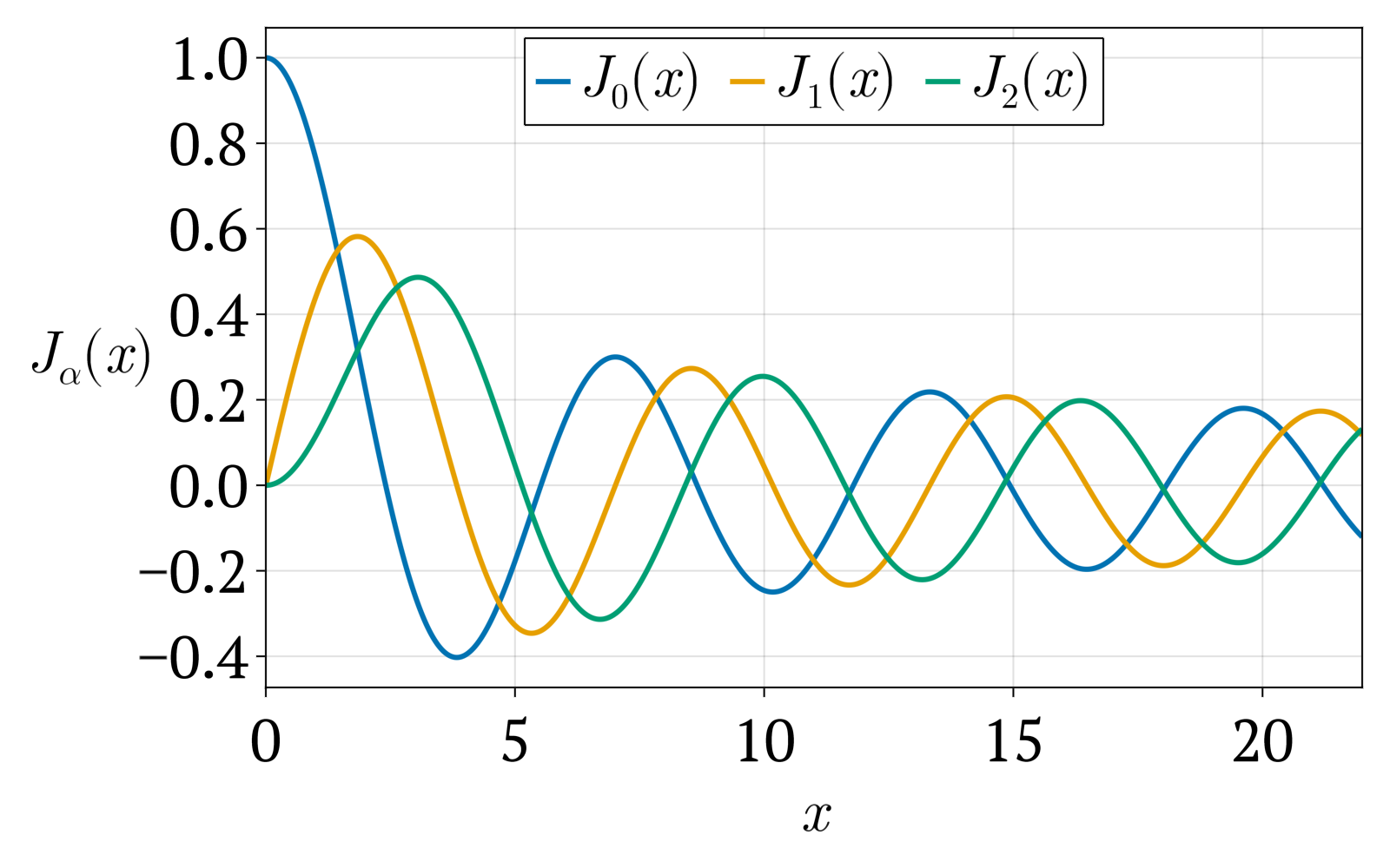
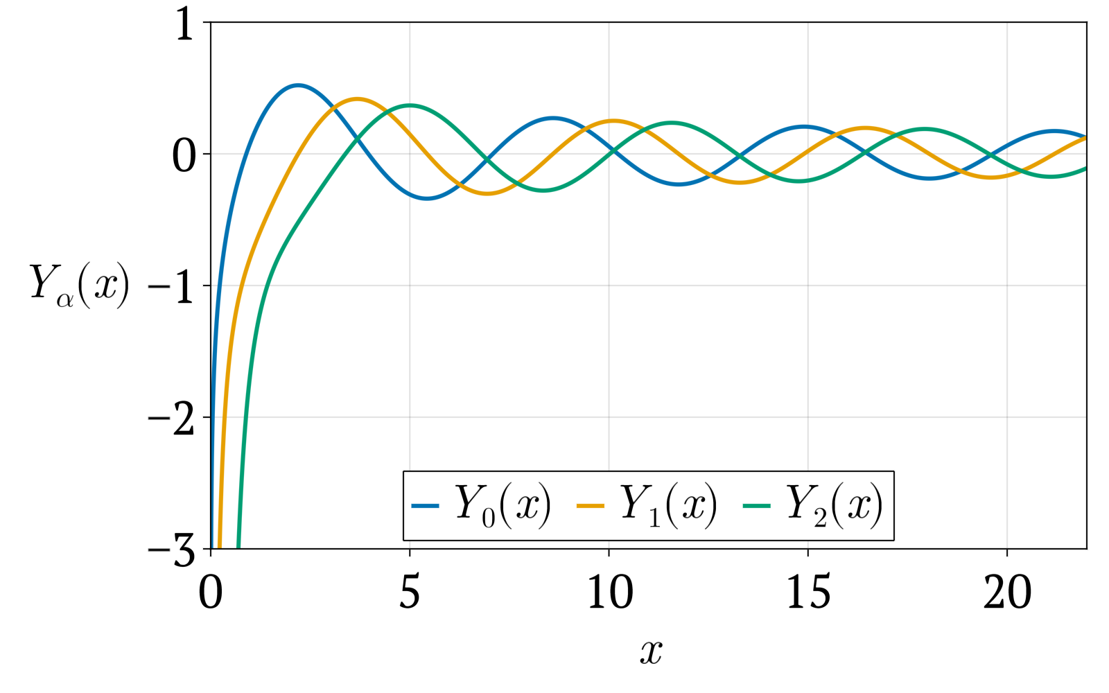
To better understand the qualitative behavior of Bessel functions, it is useful to look at their graphs. Figure 9.2 shows the first three Bessel functions of the first kind, \(J_0(x)\), \(J_1(x)\), and \(J_2(x)\), and Fig. 9.3 shows the corresponding Bessel functions of the second kind, \(Y_0(x)\), \(Y_1(x)\), and \(Y_2(x)\), all plotted for \(0<x\le 20\).

Bessel functions of the first kind J(x) for =0,1,2.
Figure 9.2. Bessel functions of the first kind \(J_\alpha(x)\) for \(\alpha=0,1,2\).
Remark - Bessel functions of the first kind \(J_\alpha(x)\)
  • \(J_0(x)\) starts from \(J_0(0)=1\); all higher orders satisfy \(J_n(0)=0\) for \(n\ge1\).

  • Each \(J_\alpha(x)\) oscillates with a wavelength that slowly approaches a constant as \(x\) increases.

  • The oscillations have a slowly decreasing amplitude, roughly decaying like \(1/\sqrt{x}\) for large \(x\).

  • The zeros of \(J_\alpha(x)\) are not equally spaced, but they become more nearly equally spaced as \(x\) grows.

  • Higher orders \(J_1(x)\), \(J_2(x),\dots\) are “pushed to the right’’: they remain small near the origin and their first zero occurs at larger values of \(x\).

Bessel functions of the second kind Y(x) for =0,1,2.
Figure 9.3. Bessel functions of the second kind \(Y_\alpha(x)\) for \(\alpha=0,1,2\).
Remark - Bessel functions of the second kind \(Y_\alpha(x)\)
  • Near the origin, all \(Y_\alpha(x)\) have a logarithmic singularity and diverge to \(-\infty\) as \(x\to0^{+}\).

  • For \(x\) away from zero, \(Y_\alpha(x)\) oscillate with a behavior similar to \(J_\alpha(x)\): approximately sinusoidal with a slowly decreasing amplitude for large \(x\).

  • Because of the divergence at \(x=0\), \(Y_\alpha(x)\) are usually not acceptable in physical problems where the solution must remain finite at the origin (for example, in cylindrical coordinates with a physical axis at \(r=0\)).

  • Nevertheless, \(Y_\alpha(x)\) form, together with \(J_\alpha(x)\), a complete set of independent solutions of Bessel’s equation on \((0,\infty)\).

9.4.8Orthogonality

On the interval \(0\le x\le R\), the Bessel functions satisfy

\begin{equation} \boxed{ \int_0^R x\, J_p\left(\alpha_{p m}\tfrac{x}{R}\right) J_p\left(\alpha_{p n}\tfrac{x}{R}\right)\,dx = \frac{R^2}{2}\,[J_{p+1}(\alpha_{p n})]^2\,\delta_{mn}, } \end{equation}

where \(\alpha_{p n}\) are the zeros of \(J_p(x)\).

Remark

This orthogonality makes Bessel functions the natural basis for expanding functions defined on circular domains, just as Legendre polynomials are the natural basis on \([-1,1]\).

9.4.9Generating Function

The Bessel functions have the elegant generating function

\begin{equation} \boxed{ e^{\frac{x}{2}(t-\frac1t)} = \sum_{n=-\infty}^{\infty} t^n J_n(x). } \end{equation}
Example

Expanding for small \(t\) yields

\begin{equation} e^{\frac{x}{2}(t-\frac1t)} = J_0(x) + tJ_1(x) + t^2 J_2(x) + \cdots + t^{-1}J_{-1}(x) + t^{-2}J_{-2}(x)+\cdots. \end{equation}

Differentiating with respect to \(t\) and evaluating at \(t=0\) (or \(\infty\)) extracts \(J_n(x)\) in the same manner as with Legendre polynomials.

9.5Orthogonal Eigenfunction Bases in Physics

We have learned that many important families of functions form orthogonal and complete bases. This means that any physically meaningful function can be expanded using these basis functions, and the expansion coefficients follow directly from their orthogonality relations.

In this section we summarize three of the most important bases encountered in mathematical physics:

\begin{equation} \boxed{ \text{Fourier series modes } e^{ik_n x},\qquad \text{Legendre polynomials } P_\ell(x),\qquad \text{Spherical harmonics } Y_{\ell m}(\theta,\phi). } \end{equation}

9.5.11. Fourier Series Modes \(e^{ik_n x}\): Basis on a Finite Interval

On the interval \(\left[-\dfrac{L}{2},\,\dfrac{L}{2}\right]\), the complex Fourier basis functions are

\begin{equation} e^{ik_n x}, \qquad k_n = \frac{2\pi n}{L}, \qquad n = 0, \pm1, \pm2, \ldots \end{equation}
Theorem - Orthogonality of the Fourier series basis
\begin{equation} \int_{-L/2}^{L/2} e^{ik_n x}\,e^{-ik_m x}\,dx = L\,\delta_{nm}. \end{equation}

Thus any function \(f(x)\) defined on \(\left[-\dfrac{L}{2},\,\dfrac{L}{2}\right]\) can be expanded as a Fourier series:

\begin{equation} f(x) = \sum_{n=-\infty}^{\infty} c_n\,e^{ik_n x}. \end{equation}

Using orthogonality, the expansion coefficients are

\begin{equation} c_n = \frac{1}{L} \int_{-L/2}^{L/2} f(x)\,e^{-ik_n x}\,dx. \end{equation}

Therefore, the set \(\{e^{ik_n x}\}\) forms a complete orthogonal basis on \(\left[-\dfrac{L}{2},\,\dfrac{L}{2}\right]\).

9.5.22. Legendre Polynomials \(P_\ell(x)\): Basis on \([-1,1]\)

When the problem depends only on an angular variable through \(x = \cos\theta\), the relevant basis functions are the Legendre polynomials:

\begin{equation} P_0(x),\,P_1(x),\,P_2(x),\ldots, \qquad -1 \le x \le 1. \end{equation}
Theorem - Orthogonality relation
\begin{equation} \int_{-1}^{1} P_\ell(x)\,P_{\ell'}(x)\,dx = \frac{2}{2\ell+1}\,\delta_{\ell\ell'}. \end{equation}

A function \(f(x)\) defined on \([-1,1]\) can be expanded as

\begin{equation} f(x) = \sum_{\ell=0}^{\infty} c_\ell\,P_\ell(x), \end{equation}

with coefficients obtained from orthogonality:

\begin{equation} c_\ell = \frac{2\ell+1}{2} \int_{-1}^{1} f(x)\,P_\ell(x)\,dx. \end{equation}

Thus \(\{P_\ell(x)\}\) forms a complete orthogonal basis on \([-1,1]\).

9.5.33. Spherical Harmonics \(Y_{\ell m}(\theta,\phi)\): Basis on the Sphere

For functions defined on the sphere, the natural basis is the set of spherical harmonics:

\begin{equation} Y_{\ell m}(\theta,\phi), \qquad \ell = 0,1,2,\ldots,\quad m=-\ell,\ldots,\ell. \end{equation}
Theorem - Orthogonality relation
\begin{equation} \int_{0}^{2\pi}\!\!\int_{0}^{\pi} Y_{\ell m}(\theta,\phi)\, Y_{\ell' m'}^{*}(\theta,\phi)\, \sin\theta\,d\theta\,d\phi = \delta_{\ell\ell'}\,\delta_{mm'}. \end{equation}

Any square-integrable function on the sphere can be expanded as

\begin{equation} f(\theta,\phi) = \sum_{\ell=0}^{\infty}\;\sum_{m=-\ell}^{\ell} c_{\ell m}\,Y_{\ell m}(\theta,\phi), \end{equation}

with expansion coefficients

\begin{equation} c_{\ell m} = \int_{0}^{2\pi}\!\!\int_{0}^{\pi} f(\theta,\phi)\,Y_{\ell m}^{*}(\theta,\phi)\, \sin\theta\,d\theta\,d\phi. \end{equation}

Thus \(\{Y_{\ell m}\}\) forms a complete orthonormal basis on the sphere \(S^{2}\).

9.6Where Series Solutions Are Used

The elementary methods of Chapter 8 fail the moment an ODE has variable coefficients, and almost every equation coming from a physical problem with spherical or cylindrical symmetry does. The power-series and Frobenius methods of this chapter are what handle them, and the special functions they produce — Legendre polynomials, Bessel functions, spherical harmonics — are not curiosities but the standard vocabulary of mathematical physics.

Remark

One structural idea ties the chapter together. Where a solution is required, an ordinary point admits an ordinary power series; a regular singular point requires the Frobenius form \(x^r\sum a_n x^n\) with \(r\) fixed by the indicial equation; an irregular singular point generally admits neither. Legendre (\(x=0\) ordinary) and Bessel (\(x=0\) regular singular) are the two worked cases, and the physically admissible solutions are singled out by demanding finiteness at the singular points — which is exactly what forces \(\ell\) to be an integer and picks \(J_p\) over \(Y_p\).

Summary Table

ObjectFormulaNotes
Ordinary pointpower series \(\sum a_n x^n\)e.g. \(x=0\) for Legendre.
Regular singular pointFrobenius \(x^r\sum a_n x^n\)\(r\) from the indicial equation; \(x=0\) for Bessel.
Legendre equation\((1-x^2)y'' - 2xy' + \ell(\ell+1)y = 0\)Finite solutions when \(\ell\in\mathbb{Z}_{\ge0}\).
Legendre recurrence\(a_{n+2} = \dfrac{n(n+1)-\ell(\ell+1)}{(n+1)(n+2)}a_n\)Terminates at \(n=\ell\), giving \(P_\ell\).
Rodrigues' formula\(P_\ell = \dfrac{1}{2^\ell \ell!}\dfrac{d^\ell}{dx^\ell}(x^2-1)^\ell\)\(P_0=1,\ P_1=x,\ P_2=\tfrac12(3x^2-1),\ldots\)
Legendre orthogonality\(\displaystyle\int_{-1}^{1} P_\ell P_{\ell'}\,dx = \dfrac{2}{2\ell+1}\delta_{\ell\ell'}\)Basis for expansions on \([-1,1]\).
Generating function\(\dfrac{1}{\sqrt{1-2xt+t^2}} = \sum_\ell P_\ell(x)t^\ell\)The multipole expansion.
Associated Legendre\(P_\ell^m = (-1)^m(1-x^2)^{m/2}\dfrac{d^m}{dx^m}P_\ell\)Angular part with azimuthal index \(m\).
Bessel equation\(x^2 y'' + xy' + (x^2-p^2)y = 0\)Regular singular point at \(x=0\).
Bessel function\(J_p(x) = \displaystyle\sum_{k=0}^{\infty}\dfrac{(-1)^k}{k!\,\Gamma(k+p+1)}\Big(\dfrac{x}{2}\Big)^{2k+p}\)Finite at \(x=0\); \(Y_p\) diverges there.
Spherical harmonics\(Y_{\ell m} = N_{\ell m}P_\ell^m(\cos\theta)e^{im\phi}\)Orthonormal basis on the sphere.

For the Interested Reader

This chapter is where a physics student first meets the special functions that recur for the rest of the subject. The two aims worth separating are learning the method (power series and Frobenius) and learning the functions (Legendre, Bessel, and their properties). The sources below split along that line. Everything is free.

The method

The functions

Remark

A practical note. In real calculations one almost never sums these series by hand; the recurrences, orthogonality integrals and generating functions of this chapter are what actually get used, and numerical libraries evaluate \(P_\ell\), \(J_p\) and \(Y_{\ell m}\) directly. The value of deriving them here is to understand why they have the properties the libraries rely on — why \(\ell\) must be an integer, why \(J_p\) and not \(Y_p\) is finite at the origin, and why the expansions converge.