Chapter 8

Ordinary Differential Equations

8.1Introduction and General Form

An ordinary differential equation (ODE) is an equation that relates a function $$y(x)$$ to its derivatives with respect to a single independent variable $$x$$ :

\begin{equation} F\!\left(x, y, \frac{dy}{dx}, \frac{d^2y}{dx^2}, \ldots, \frac{d^n y}{dx^n}\right) = 0. \end{equation}

Example - Second-order ordinary differential equation

\begin{equation} x^2 \frac{d^2y}{dx^2} + 3x \frac{dy}{dx} + y = 0. \end{equation}

Definition - Basic Terminology for ODEs

Order of an ODE: The order of a differential equation is the highest derivative that appears in the equation.
$\begin{equation} \frac{d^3y}{dx^3} + 2\frac{dy}{dx} = 0 \quad \Rightarrow \quad \text{Order} = 3 \end{equation}$
Degree of an ODE: The degree of a differential equation is the exponent of the highest-order derivative, provided the equation is polynomial in derivatives.
$\begin{equation} \left(\frac{d^2y}{dx^2}\right)^3 + \frac{dy}{dx} = 0 \quad \Rightarrow \quad \text{Degree} = 3 \end{equation}$
Solution of an ODE: A function $$y(x)$$ that satisfies the differential equation for all $$x$$ in a given interval.
$\begin{equation} \frac{dy}{dx} = 2x \quad \Rightarrow \quad y = x^2 + C \end{equation}$

8.2Classification of ODEs

Ordinary differential equations (ODEs) can be classified according to several characteristics. The most fundamental distinction is between linear and nonlinear equations.

Linear vs. Nonlinear ODEs

An ODE is called linear if the dependent variable $$y$$ and all its derivatives appear only to the first power and are not multiplied or composed with each other. The general $n^{\text{th}}$ -order linear ODE can be written as

\begin{equation} a_n(x)\,y^{(n)} + a_{n-1}(x)\,y^{(n-1)} + \cdots + a_1(x)\,y' + a_0(x)\,y = f(x), \end{equation}

where $$a_i(x)$$ and $$f(x)$$ are known functions of the independent variable $$x$$ .

If any term involves products or nonlinear functions of $$y$$ or its derivatives (such as $$y^2$$ , $y\,y'$ , or $\sin y$ ), the equation is said to be nonlinear.

Example

\begin{align*} \text{Linear:} \quad & y'' + 3y' + 2y = \sin x, \\[4pt] \text{Nonlinear:} \quad & y'' + y\,y' = 0. \end{align*}

Remark

Linear ODEs are generally easier to solve because they obey the principle of superposition, if $$y_1$$ and $$y_2$$ are solutions, then any linear combination $$C_1 y_1 + C_2 y_2$$ is also a solution. Nonlinear ODEs, on the other hand, can exhibit far richer behavior, such as limited analytic solvability, sensitivity to initial conditions, or even chaotic motion. However, certain first-order nonlinear equations, such as separable or Bernoulli equations, can still be solved analytically.

Classification of Linear ODEs

Once an equation is identified as linear, we can further classify it based on its right-hand side and coefficients.

Homogeneous Linear ODE: The right-hand side equals zero,
$\begin{equation} a_n(x)\,y^{(n)} + a_{n-1}(x)\,y^{(n-1)} + \cdots + a_0(x)\,y = 0. \end{equation}$
In this case, every term involves $$y$$ or its derivatives, and the trivial solution $$y=0$$ always satisfies the equation. The general solution typically involves $$n$$ arbitrary constants determined by initial or boundary conditions.
Nonhomogeneous Linear ODE: The right-hand side is a nonzero function $$f(x)$$ ,
$\begin{equation} a_n(x)\,y^{(n)} + a_{n-1}(x)\,y^{(n-1)} + \cdots + a_0(x)\,y = f(x). \end{equation}$
The general solution is the sum of two parts:
$\begin{equation} \boxed{y(x) = y_h(x) + y_p(x)}, \end{equation}$
where $$y_h$$ is the general solution of the corresponding homogeneous equation and $$y_p$$ is a particular solution to the full nonhomogeneous equation.
Linear ODEs with Constant Coefficients: When the coefficients $$a_i$$ are constants rather than functions of $$x$$ ,
$\begin{equation} a_n\,y^{(n)} + a_{n-1}\,y^{(n-1)} + \cdots + a_1\,y' + a_0\,y = f(x), \end{equation}$
the equation becomes especially important in physics and engineering. Such forms describe systems like simple harmonic oscillators, RC and RL circuits, and exponential decay processes.

8.3First-Order ODEs

A first-order ODE involves only the first derivative of the unknown function:

\begin{equation} \frac{dy}{dx} = f(x, y). \end{equation}

This general form can represent both linear and nonlinear cases, depending on how $$f(x, y)$$ depends on $$y$$ . Such equations appear widely in physics—for example, in modeling exponential decay, population growth, or motion with velocity-dependent forces.

8.3.1Separable Equations

A first-order ODE is called separable if it can be expressed as

\begin{equation} \frac{dy}{dx} = g(x)\,h(y), \end{equation}

where the function on the right-hand side is the product of a function of $$x$$ and a function of $$y$$ . Although separable equations are often nonlinear, they are still analytically solvable because the variables can be separated.

Rearranging terms gives

\begin{equation} \frac{dy}{h(y)} = g(x)\,dx, \end{equation}

and integrating both sides yields

\begin{equation} \int \frac{dy}{h(y)} = \int g(x)\,dx. \end{equation}

Example - Solve the differential equation

\begin{equation} \frac{dy}{dx} = x\,y. \end{equation}

Solution.

Step 1. Recognize the type of equation. This is a first-order separable (and also linear) differential equation.

Step 2. Separate the variables.

\begin{equation} \frac{dy}{y} = x\,dx. \end{equation}

Step 3. Integrate both sides.

\begin{equation} \int \frac{1}{y}\,dy = \int x\,dx \quad\Longrightarrow\quad \ln|y| = \frac{x^{2}}{2} + C. \end{equation}

Step 4. Simplify the result. Exponentiate both sides:

\begin{equation} y = e^{C}\,e^{x^{2}/2}. \end{equation}

Let $C_1 = e^{C}$ (a new arbitrary constant). Then

\begin{equation} \boxed{y(x) = C_1 e^{x^{2}/2}}. \end{equation}

Step 5. Verification. Differentiate $y = C_1 e^{x^{2}/2}$ :

\begin{equation} \frac{dy}{dx} = C_1\,x\,e^{x^{2}/2} = x\,y, \end{equation}

confirming that the solution satisfies the ODE.

Example - Solve the differential equation

\begin{equation} x\,\frac{dy}{dx} = y + 1. \end{equation}

Solution.

Step 1. Separate the variables. Divide both sides by $$x(y+1)$$ :

\begin{equation} \frac{1}{y+1}\frac{dy}{dx} = \frac{1}{x} \quad\Longrightarrow\quad \frac{dy}{y+1} = \frac{dx}{x}. \end{equation}

Step 2. Integrate both sides.

\begin{equation} \int \frac{dy}{y+1} = \int \frac{dx}{x} \quad\Longrightarrow\quad \ln|y+1| = \ln|x| + C. \end{equation}

Step 3. Simplify the constant. Let $C = \ln a$ (for $$a>0$$ ) to combine logarithms conveniently:

\begin{equation} \ln|y+1| = \ln|a x|. \end{equation}

Step 4. Remove the logarithms.

\begin{equation} |y+1| = a|x|. \end{equation}

Because $$a$$ can absorb the sign, we write simply

\begin{equation} \boxed{\,y + 1 = a x\,}, \qquad a \text{ constant}. \end{equation}

Step 5. Interpretation. The general solution

\begin{equation} y = a x - 1 \end{equation}

represents a family of straight lines in the $$(x,y)$$ -plane, one line for each value of the constant $$a$$ . Selecting a particular value of $$a$$ determines a single specific curve from this family.

Example - Solve the differential equation

\begin{equation} \frac{dy}{dx} = \sqrt{\,1 - y^2\,}. \end{equation}

Find the particular solutions satisfying (a) $$x=0, y=0$$ and (b) $$x=0, y=1$$ , and discuss any solutions not obtained by separation.

Solution.

Step 1. Separation of variables and integration. For $$|y| < 1$$ , the equation can be written in separable form:

\begin{equation} \frac{dy}{\sqrt{1 - y^2}} = dx. \end{equation}

Integrating both sides gives

\begin{equation} \arcsin(y) = x + \alpha, \end{equation}

so the general solution (valid where $$|y|<1$$ ) is

\begin{equation} \boxed{y(x) = \sin(x + \alpha)}. \end{equation}

Step 2. Monotonicity and physical interpretation. Since $y' = \sqrt{1 - y^2} \ge 0$ , the slope of the curve is always nonnegative. Hence, only the increasing portions of the sine curve correspond to valid solution segments. That is, we must restrict to intervals where

\begin{equation} \cos(x + \alpha) \ge 0. \end{equation}

The figure below shows the slope field and the increasing sine segments that satisfy this condition.

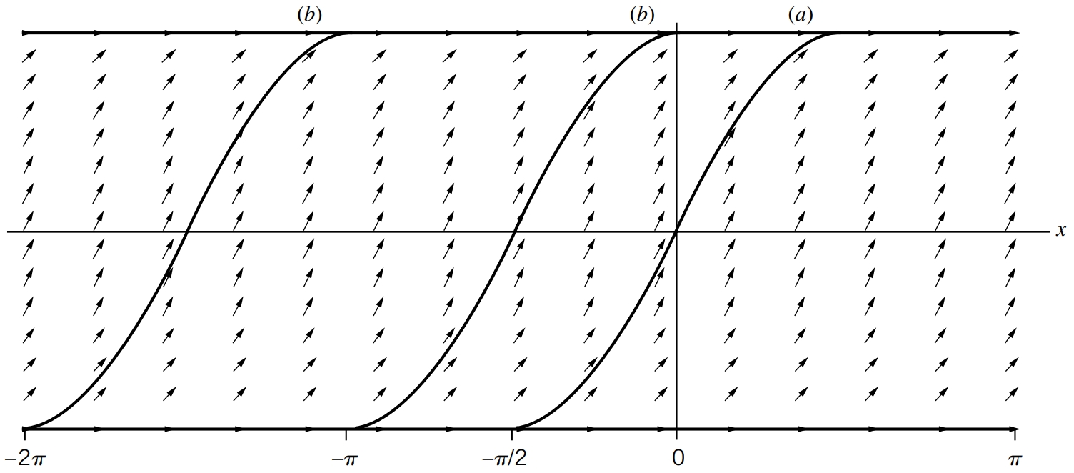
The slope field with the increasing segments of the sine curve, which are the parts that satisfy (x+) 0. — Figure 8.1. The slope field with the increasing segments of the sine curve, which are the parts that satisfy $\cos(x+\alpha)\ge 0$ .

Step 3. Singular (boundary) solutions. In separating variables, we divided by $\sqrt{1 - y^2}$ , which is not defined when $$|y| = 1$$ . However, substituting directly into the differential equation shows that

\begin{equation} y \equiv 1, \qquad y \equiv -1 \end{equation}

are valid constant solutions since $y' = 0 = \sqrt{1 - y^2}$ . These are singular solutions that cannot be obtained from the separated form.

Step 4. Particular solutions.

(a) $$y(0)=0$$ : From $\arcsin y = x + \alpha$ , substituting $x=0,\, y=0$ gives $\alpha=0$ or $\pi$ . Because $y'\ge 0$ , we take the increasing branch:

\begin{equation} \boxed{y(x) = \sin x, \qquad -\frac{\pi}{2} \le x \le \frac{\pi}{2}.} \end{equation}

To extend this continuously for all $$x$$ , attach the constant segments $y = \pm 1$ :

\begin{equation} y(x) = \begin{cases} -1, & x \le -\dfrac{\pi}{2},\\[4pt] \sin x, & -\dfrac{\pi}{2} \le x \le \dfrac{\pi}{2},\\[4pt] 1, & x \ge \dfrac{\pi}{2}. \end{cases} \end{equation}

This gives a single continuous nondecreasing solution over the entire real line.

(b) $$y(0)=1$$ : The constant function $y(x)\equiv1$ is an obvious solution. Alternatively, using $\sin(x+\alpha)=1$ at $$x=0$$ gives $\alpha=\dfrac{\pi}{2}+2k\pi$ . Choosing the increasing branch near $$x=0$$ ,

\begin{equation} \boxed{y(x) = \sin\!\Big(x + \frac{\pi}{2}\Big) = \cos x, \qquad -\pi \le x \le 0.} \end{equation}

To extend for all $$x$$ :

\begin{equation} y(x) = \begin{cases} -1, & x \le -\pi,\\[4pt] \cos x, & -\pi \le x \le 0,\\[4pt] 1, & x \ge 0. \end{cases} \end{equation}

There exist infinitely many such piecewise continuous solutions, obtained by shifting these arcs horizontally.

Step 5. Interpretation and summary.

The general solution $y = \sin(x+\alpha)$ applies where $$|y|<1$$ and $y' = \sqrt{1-y^2} \ge 0$ .
The singular solutions $y = \pm1$ correspond to the flat portions of the slope field where $$y'=0$$ .
The complete solution set consists of rising sine arcs smoothly connected to horizontal segments at $y=\pm1$ .

All solutions.

y(x) = (x+) on intervals where (x+)0, together with y1.

8.3.2Linear First-Order Equations

A linear first-order equation has the form

\begin{equation} \frac{dy}{dx} + P(x)y = Q(x). \end{equation}

Integrating Factor Method:

Compute the integrating factor:
$\begin{equation} \mu(x) = e^{\int P(x)\,dx}. \end{equation}$
Multiply through by $\mu(x)$ :
$\begin{equation} \frac{d}{dx}\!\left(\mu(x)y\right) = \mu(x)Q(x). \end{equation}$
Integrate:
$\begin{equation} \mu(x)y = \int \mu(x)Q(x)\,dx. \end{equation}$
Solve for $$y(x)$$ :
$\begin{equation} \boxed{y = [\mu(x)]^{-1} \int \mu(x) Q(x)\,dx}. \end{equation}$

Example - Solve the first-order linear ODE

\begin{equation} y' + 2y = e^{-x}. \end{equation}

Solution.

Step 1. Identify $$P(x)$$ and $$Q(x)$$ . The equation is in the standard linear form

\begin{equation} y' + P(x)y = Q(x), \end{equation}

where

\begin{equation} P(x) = 2, \qquad Q(x) = e^{-x}. \end{equation}

Step 2. Compute the integrating factor. The integrating factor is

\begin{equation} \mu(x) = e^{\int P(x)\,dx} = e^{\int 2\,dx} = e^{2x}. \end{equation}

Step 3. Apply the general solution formula.

\begin{equation} \boxed{ y = [\mu(x)]^{-1} \int \mu(x) Q(x)\,dx. } \end{equation}

Substitute $\mu(x) = e^{2x}$ and $Q(x) = e^{-x}$ :

\begin{equation} y = e^{-2x}\int e^{2x} e^{-x}\,dx = e^{-2x}\int e^{x}\,dx. \end{equation}

Step 4. Evaluate the integral.

\begin{equation} y = e^{-2x}(e^{x} + C) = e^{-x} + C e^{-2x}. \end{equation}

Final Answer:

\begin{equation} \boxed{y = e^{-x} + C e^{-2x}.} \end{equation}

Verification. Substitute $y = e^{-x} + C e^{-2x}$ into the original equation:

\begin{equation} y' = -e^{-x} - 2C e^{-2x}, \quad\Rightarrow\quad y' + 2y = (-e^{-x} - 2C e^{-2x}) + 2(e^{-x} + C e^{-2x}) = e^{-x}, \end{equation}

which satisfies the ODE.

Separable equations and linear equations are the two types of first-order equations most commonly encountered in basic applications. However, there exist several other important forms of first-order equations that can be transformed into solvable types. In this section, we briefly introduce two such forms: the Bernoulli equation and exact equations. More details and applications are found in advanced differential equations texts.

8.3.4The Bernoulli Equation

The differential equation

\begin{equation} y' + P(x)y = Q(x)y^n, \end{equation}

where $$P(x)$$ and $$Q(x)$$ are known functions of $$x$$ , is called the Bernoulli equation. It is nonlinear for $n \neq 0, 1$ , but it can be transformed into a linear equation through an appropriate substitution.

Step 1. Multiply by $y^{-n}$ .

\begin{equation} y^{-n}y' + P(x)y^{1-n} = Q(x). \end{equation}

Step 2. Simplify using the substitution $z = y^{1-n}$ .

\begin{equation} \frac{dz}{dx} = (1-n)y^{-n}y'. \end{equation}

Hence, $y^{-n}y' = \dfrac{1}{1-n}\,z'$ . Substitute this into the previous equation:

\begin{equation} \dfrac{1}{1-n}z' + P(x)z = Q(x). \end{equation}

Step 3. Multiply through by $$(1-n)$$ to simplify.

\begin{equation} z' + (1-n)P(x)z = (1-n)Q(x). \end{equation}

This is now a first-order linear ODE in $$z(x)$$ , which can be solved using the integrating factor method.

Reduced linear form: z' + (1-n)P(x)z = (1-n)Q(x).

After solving for $$z(x)$$ , the original dependent variable is recovered via

\begin{equation} y = z^{\frac{1}{1-n}}. \end{equation}

Remark

The Bernoulli equation provides an important link between nonlinear and linear first-order ODEs. By multiplying through by $y^{-n}$ and substituting $z = y^{1-n}$ , we convert a nonlinear equation into a solvable linear form. This transformation frequently appears in problems involving population dynamics, exponential growth and decay, and fluid motion.

Example - Reduce to linear form and solve

\begin{equation} y' + y = x\,y^{2/3}. \end{equation}

Solution.

Step 1. Multiply by $y^{-n}$ with $n=\tfrac{2}{3}$ .

\begin{equation} y^{-2/3}y' + y^{1/3} = x. \end{equation}

Step 2. Let $z = y^{1-n}=y^{1/3}$ . Then $z'=\tfrac{1}{3}y^{-2/3}y'$ , so $y^{-2/3}y'=3z'$ . Substitute:

\begin{equation} 3z' + z = x \quad\Longrightarrow\quad z' + \tfrac{1}{3}z = \tfrac{1}{3}x. \end{equation}

Step 3. Solve the linear equation using the integrating-factor formula. For

\begin{equation} z' + p(x)z = q(x), \qquad p(x)=\tfrac{1}{3},\; q(x)=\tfrac{1}{3}x, \end{equation}

the integrating factor is $\mu(x)=e^{\int p(x)\,dx}=e^{x/3}$ . Apply

\begin{equation} \boxed{\,z = [\mu(x)]^{-1}\int \mu(x)\,q(x)\,dx\,}: \end{equation}

\begin{equation} z = e^{-x/3}\left[\int e^{x/3}\cdot \tfrac{1}{3}x\,dx + C\right] = e^{-x/3}\big[e^{x/3}(x-3)+C\big] = x-3 + C e^{-x/3}. \end{equation}

Step 4. Back–substitute to $$y$$ . Since $z=y^{1/3}$ ,

\begin{equation} \boxed{\,y(x)=\big(x-3 + C e^{-x/3}\big)^{3}\,}. \end{equation}

Step 5. Singular solution. Because $y^{2/3}\ge 0$ for all real $$y$$ , the constant function

\begin{equation} \boxed{\,y(x)\equiv 0\,} \end{equation}

also satisfies the original ODE. Thus the complete set consists of the one-parameter family above together with $y\equiv 0$ .

8.3.5Exact Differential Equations

A general first-order differential equation can often be written in the form

\begin{equation} M(x,y)\,dx + N(x,y)\,dy = 0, \end{equation}

where $$M$$ and $$N$$ are functions of two variables $$x$$ and $$y$$ .

Definition - Exact Differential Equation

The first–order differential equation

\begin{equation} M(x,y)\,dx + N(x,y)\,dy = 0 \end{equation}

is called exact if there exists a scalar function $$U(x,y)$$ (called a potential function) such that

\begin{equation} dU(x,y) = M(x,y)\,dx + N(x,y)\,dy, \qquad \text{where } M = \frac{\partial U}{\partial x}, \quad N = \frac{\partial U}{\partial y}. \end{equation}

In this case, the general solution can be written implicitly as

\begin{equation} U(x,y) = C. \end{equation}

A necessary and sufficient condition for exactness (assuming continuous partial derivatives) is

\begin{equation} \boxed{\frac{\partial M}{\partial y} = \frac{\partial N}{\partial x}}. \end{equation}

Remark

The condition above ensures that the mixed second derivatives of $$U(x,y)$$ are equal:

\begin{equation} \frac{\partial^2 U}{\partial x \partial y} = \frac{\partial^2 U}{\partial y \partial x}. \end{equation}

This is guaranteed by Clairaut’s theorem when $$M$$ and $$N$$ have continuous partial derivatives.

Solution Procedure:

Check whether $\dfrac{\partial M}{\partial y} = \dfrac{\partial N}{\partial x}$ . If true, the equation is exact.
Integrate $$M(x,y)$$ with respect to $$x$$ , treating $$y$$ as constant:
$\begin{equation} U(x,y) = \int M(x,y)\,dx + F(y), \end{equation}$
where $$F(y)$$ is an arbitrary function of $$y$$ .
Since $$U(x,y)$$ must satisfy
$\begin{equation} \boxed{\,N(x,y) = \frac{\partial U}{\partial y}\,}, \end{equation}$
we differentiate the above expression for $$U(x,y)$$ with respect to $$y$$ :
$\begin{equation} \frac{\partial U}{\partial y} = \frac{\partial}{\partial y}\!\left(\int M(x,y)\,dx\right) + F'(y). \end{equation}$
Now substitute the known expression for $$N(x,y)$$ from the original equation and equate:
$\begin{equation} N(x,y) = \frac{\partial}{\partial y}\!\left(\int M(x,y)\,dx\right) + F'(y). \end{equation}$
From this, we can solve for $$F'(y)$$ :
$\begin{equation} F'(y) = N(x,y) - \frac{\partial}{\partial y}\!\left(\int M(x,y)\,dx\right). \end{equation}$
Integrate with respect to $$y$$ to find $$F(y)$$ , and then write the final expression for $$U(x,y)$$ . The general solution is obtained from
$\begin{equation} \boxed{\,U(x,y) = \text{constant.}\,} \end{equation}$
Integrate $$F'(y)$$ to find $$F(y)$$ , substitute back, and write the final solution $$U(x,y) = C$$ .

Example - Solving an Exact Differential Equation

Solve

\begin{equation} (2xy + y^3)\,dx + (x^2 + 3xy^2)\,dy = 0. \end{equation}

Solution.

Step 1. Identify

\begin{equation} M(x,y) = 2xy + y^3, \qquad N(x,y) = x^2 + 3xy^2. \end{equation}

Step 2. Check the exactness condition:

\begin{equation} \frac{\partial M}{\partial y} = 2x + 3y^2, \qquad \frac{\partial N}{\partial x} = 2x + 3y^2. \end{equation}

They are equal, so the equation is exact.

Step 3. Integrate $$M(x,y)$$ with respect to $$x$$ :

\begin{equation} U(x,y) = \int (2xy + y^3)\,dx = x^2y + x y^3 + F(y). \end{equation}

Step 4. Differentiate with respect to $$y$$ :

\begin{equation} \frac{\partial U}{\partial y} = x^2 + 3x y^2 + F'(y). \end{equation}

Compare with $$N(x,y) = x^2 + 3x y^2$$ , which implies $$F'(y)=0$$ .

Step 5. Hence $F(y)=\text{constant}$ . The potential function is

\begin{equation} U(x,y) = x^2y + x y^3. \end{equation}

Step 6. The general solution is

\begin{equation} \boxed{x^2y + xy^3 = C.} \end{equation}

8.3.6Integrating Factors

If the equation $M(x,y)\,dx + N(x,y)\,dy = 0$ is not exact, it may sometimes be made exact by multiplying by a function $\mu(x,y)$ called an integrating factor:

\begin{equation} \mu(x,y)\,M(x,y)\,dx + \mu(x,y)\,N(x,y)\,dy = 0. \end{equation}

The new equation is exact if

\begin{equation} \frac{\partial (\mu M)}{\partial y} = \frac{\partial (\mu N)}{\partial x}. \end{equation}

Unfortunately, there is no universal method for finding $\mu(x,y)$ . However, there are two common and important special cases.

Case 1: Integrating factor depends on $$x$$ only.

If $\mu = \mu(x)$ , then the equation becomes exact provided that

\begin{equation} \frac{1}{\mu}\frac{d\mu}{dx} = \frac{\frac{\partial M}{\partial y} - \frac{\partial N}{\partial x}}{N}. \end{equation}

Hence,

\begin{equation} \mu(x) = \exp\!\left(\int \frac{1}{N}\Big(\frac{\partial M}{\partial y} - \frac{\partial N}{\partial x}\Big)\,dx\right). \end{equation}

Case 2: Integrating factor depends on $$y$$ only.

If $\mu = \mu(y)$ , then the equation becomes exact provided that

\begin{equation} \frac{1}{\mu}\frac{d\mu}{dy} = \frac{\frac{\partial N}{\partial x} - \frac{\partial M}{\partial y}}{M}. \end{equation}

Hence,

\begin{equation} \mu(y) = \exp\!\left(\int \frac{1}{M}\Big(\frac{\partial N}{\partial x} - \frac{\partial M}{\partial y}\Big)\,dy\right). \end{equation}

Example - Integrating factor

\mu=\mu(x)

, not separable

Solve

\begin{equation} \bigl[(x+1)\,y + x\bigr]\,dx + x\,dy = 0. \end{equation}

Solution.

Step 1. Identify $$M,N$$ and test exactness.

\begin{equation} M(x,y)=(x+1)\,y + x,\qquad N(x,y)=x. \end{equation}

Compute

\begin{equation} M_y = x+1,\qquad N_x=1. \end{equation}

Since $M_y\neq N_x$ , the equation is not exact.

Step 2. Seek an integrating factor $\mu=\mu(x)$ . Use

\begin{equation} \frac{1}{\mu}\frac{d\mu}{dx}=\frac{M_y-N_x}{N} =\frac{(x+1)-1}{x}=\frac{x}{x}=1. \end{equation}

Hence

\begin{equation} \ln\mu(x)=\int 1\,dx=x \quad\Rightarrow\quad \boxed{\mu(x)=e^{x}}. \end{equation}

Step 3. Multiply the equation by $\mu(x)=e^x$ .

\begin{equation} e^x\bigl[(x+1)\,y + x\bigr]\,dx + e^x x\,dy=0. \end{equation}

Define

\begin{equation} \tilde M=e^x\bigl[(x+1)\,y + x\bigr],\qquad \tilde N=e^x x. \end{equation}

Step 4. Check exactness \& find a potential $$U(x,y)$$ .

\begin{equation} \frac{\partial \tilde M}{\partial y}=e^x(x+1),\qquad \frac{\partial \tilde N}{\partial x}=e^x(x+1)\;\Rightarrow\;\text{exact}. \end{equation}

Integrate $\tilde M$ w.r.t. $$x$$ (treating $$y$$ constant):

\begin{equation} U(x,y)=\int e^x\bigl[(x+1)\,y + x\bigr]\,dx = y\!\int e^x(x+1)\,dx + \int x e^x\,dx. \end{equation}

Using $\int e^x(x+1)\,dx = x e^x$ and $\int x e^x\,dx=(x-1)e^x$ ,

\begin{equation} U(x,y)=y\,x e^x + (x-1)e^x + F(y). \end{equation}

Now

\begin{equation} U_y = x e^x + F'(y) \stackrel{!}{=} \tilde N = x e^x \;\Rightarrow\; F'(y)=0 \Rightarrow F(y)=\text{const}. \end{equation}

Step 5. Implicit solution.

\begin{equation} \boxed{\,e^x\bigl(xy + x - 1\bigr)=C.\,} \end{equation}

Example - Integrating factor

\mu=\mu(y)

, not separable

Solve

\begin{equation} y\,dx + (3x + y)\,dy = 0. \end{equation}

Solution.

Step 1. Identify $$M,N$$ and test exactness.

\begin{equation} M(x,y)=y,\qquad N(x,y)=3x + y. \end{equation}

Compute

\begin{equation} M_y=1,\qquad N_x=3. \end{equation}

Since $M_y\neq N_x$ , the equation is not exact.

Step 2. Seek an integrating factor $\mu=\mu(y)$ . Use

\begin{equation} \frac{1}{\mu}\frac{d\mu}{dy}=\frac{N_x - M_y}{M} =\frac{3-1}{y}=\frac{2}{y}. \end{equation}

Hence

\begin{equation} \ln\mu(y)=\int \frac{2}{y}\,dy = 2\ln|y| \quad\Rightarrow\quad \boxed{\mu(y)=y^{2}}\quad (y\neq 0). \end{equation}

Step 3. Multiply the equation by $\mu(y)=y^2$ .

\begin{equation} y^3\,dx + \bigl(3x y^2 + y^3\bigr)\,dy = 0. \end{equation}

Define

\begin{equation} \tilde M = y^3,\qquad \tilde N = 3x y^2 + y^3. \end{equation}

Step 4. Check exactness \& find a potential $$U(x,y)$$ .

\begin{equation} \frac{\partial \tilde M}{\partial y} = 3y^2,\qquad \frac{\partial \tilde N}{\partial x} = 3y^2 \;\Rightarrow\;\text{exact}. \end{equation}

Integrate $\tilde M$ w.r.t. $$x$$ (treating $$y$$ constant):

\begin{equation} U(x,y) = \int y^3\,dx = x y^3 + F(y). \end{equation}

Now

\begin{equation} U_y = 3x y^2 + F'(y) \stackrel{!}{=} \tilde N = 3x y^2 + y^3 \;\Rightarrow\; F'(y)=y^3 \Rightarrow F(y)=\frac{y^4}{4}. \end{equation}

Step 5. Implicit solution.

\begin{equation} \boxed{\,x\,y^{3} + \frac{y^{4}}{4} = C.\,} \end{equation}

Remark

Many physical systems—such as thermodynamics, potential flow, and electrostatics—lead to exact differential equations, where $$U(x,y)$$ represents a potential energy, enthalpy, or potential function. When the equation is not exact, an integrating factor often restores this structure.

8.4Second-Order Ordinary Differential Equations

A second-order linear ordinary differential equation (ODE) has the general form

\begin{equation} a_2(x)\,y'' + a_1(x)\,y' + a_0(x)\,y = f(x), \end{equation}

where $$a_2(x), a_1(x), a_0(x)$$ , and $$f(x)$$ are known functions of $$x$$ , and $$y(x)$$ is the unknown function to be determined.

When $$a_2,a_1,a_0$$ are constants, the equation simplifies to

\begin{equation} a\,y'' + b\,y' + c\,y = f(x), \qquad a,b,c\in\mathbb{R}, \ a\neq0. \end{equation}

We will first study the homogeneous case ( $$f(x)=0$$ ) and then the nonhomogeneous case ( $f(x)\neq0$ ).

8.4.1Homogeneous Equations with Constant Coefficients

Definition - Homogeneous Linear ODE (Second Order)

A second–order homogeneous linear differential equation with constant coefficients has the form

\begin{equation} a\,y'' + b\,y' + c\,y = 0, \qquad a, b, c \in \mathbb{R}, \ a \ne 0. \end{equation}

Theorem - General Solution of a Constant–Coefficient ODE

Consider the homogeneous linear differential equation

\begin{equation} a\,y'' + b\,y' + c\,y = 0, \qquad a \neq 0. \end{equation}

Its solutions are determined by the characteristic (auxiliary) equation

\begin{equation} a r^{2} + b r + c = 0. \end{equation}

If $$r_1$$ and $$r_2$$ are the roots of this quadratic, then the general solution is:

\begin{equation} \boxed{ \begin{aligned} \text{(i) Distinct real roots } r_1 \neq r_2: &\quad y(x) = C_1 e^{r_1 x} + C_2 e^{r_2 x}, \\[6pt] \text{(ii) Repeated root } r_1 = r_2 = r: &\quad y(x) = (C_1 + C_2 x)\,e^{r x}, \\[6pt] \text{(iii) Complex roots } r = \alpha \pm i\beta: &\quad y(x) = e^{\alpha x}\!\left(C_1 \cos(\beta x) + C_2 \sin(\beta x)\right), \end{aligned}} \end{equation}

where $$C_1, C_2$$ are arbitrary constants.

Consider the homogeneous constant–coefficient ODE

\begin{equation} a\,y''+b\,y'+c\,y=0,\qquad a\neq 0. \end{equation}

Step 1: Exponential trial and substitution. Assume a trial solution $y=e^{r x}$ with constant $$r$$ . Then

\begin{equation} y' = r e^{r x},\qquad y'' = r^2 e^{r x}. \end{equation}

Substituting into the ODE gives

\begin{equation} a (r^2 e^{r x}) + b (r e^{r x}) + c (e^{r x}) \;=\; e^{r x}\big(a r^2 + b r + c\big)\;=\;0. \end{equation}

Since $e^{r x}\neq 0$ for all $$x$$ , we must have the characteristic equation

\begin{equation} \boxed{\,a r^2 + b r + c = 0.\,} \end{equation}

Step 2: Distinct real roots $r_1\neq r_2$ . If the characteristic polynomial has two distinct real roots $$r_1$$ and $$r_2$$ , then

\begin{equation} y_1=e^{r_1 x}, \qquad y_2=e^{r_2 x} \end{equation}

are both solutions. Their Wronskian is

\begin{equation} W[y_1,y_2](x)= \begin{vmatrix} e^{r_1 x} & e^{r_2 x}\\ r_1 e^{r_1 x} & r_2 e^{r_2 x} \end{vmatrix} = (r_2-r_1)\,e^{(r_1+r_2)x}\neq 0, \end{equation}

so $$y_1,y_2$$ are linearly independent. Hence the general solution is

\begin{equation} y(x)=C_1 e^{r_1 x}+C_2 e^{r_2 x}. \end{equation}

Step 3: Repeated real root $$r_1=r_2=r$$ . (Construction of the $x e^{r x}$ term.) If the characteristic polynomial has a double root $$r$$ , then we already have one solution $y_1=e^{r x}$ . To find a second, linearly independent solution, set

\begin{equation} y_2(x)=v(x)\,e^{r x}, \end{equation}

where $$v$$ is to be determined. Compute derivatives:

\begin{equation} y_2' = v' e^{r x} + r v e^{r x},\qquad y_2'' = v'' e^{r x} + 2 r v' e^{r x} + r^2 v e^{r x}. \end{equation}

Substitute $$y_2,y_2',y_2''$$ into the ODE:

\begin{equation} a\big(v'' + 2 r v' + r^2 v\big)e^{r x} + b\big(v' + r v\big)e^{r x} + c\big(v\big)e^{r x} = 0. \end{equation}

Divide by $e^{r x}\neq 0$ and group terms by $$v'', v', v$$ :

\begin{equation} a v'' + (2 a r + b) v' + (a r^2 + b r + c)\,v = 0. \end{equation}

Because $$r$$ is a root of the characteristic polynomial, we have

\begin{equation} a r^2 + b r + c = 0. \end{equation}

Moreover, because the root is repeated, the derivative of the characteristic polynomial also vanishes at $$r$$ :

\begin{equation} \frac{d}{dr}(a r^2+br+c)\Big|_{r} = 2 a r + b = 0. \end{equation}

Hence the equation for $$v$$ reduces to

\begin{equation} a\,v'' = 0 \quad\Rightarrow\quad v''=0 \quad\Rightarrow\quad v(x)=A x + B. \end{equation}

Discarding the multiple of the first solution (the $B e^{r x}$ part), we take $$v(x)=x$$ and obtain

\begin{equation} \boxed{\,y_2(x)=x e^{r x}\,}. \end{equation}

Therefore, the general solution in the repeated-root case is

\begin{equation} y(x)=(C_1 + C_2 x)e^{r x}. \end{equation}

Step 4: Complex conjugate roots $r=\alpha\pm i\beta$ with $\beta\neq 0$ . If $r=\alpha\pm i\beta$ , then $e^{(\alpha\pm i\beta)x}$ are solutions. Taking real and imaginary parts,

\begin{equation} e^{\alpha x}\cos(\beta x),\qquad e^{\alpha x}\sin(\beta x) \end{equation}

are real solutions. Their Wronskian is

\begin{equation} W\big[e^{\alpha x}\cos\beta x,\, e^{\alpha x}\sin\beta x\big] = \beta\,e^{2\alpha x}\neq 0, \end{equation}

so they are linearly independent. Thus the general real solution is

\begin{equation} y(x)=e^{\alpha x}\big(C_1\cos\beta x + C_2\sin\beta x\big). \end{equation}

Combining the three cases completes the proof.

Remark

The step $$2ar+b=0$$ in the repeated-root case is precisely the condition $$p'(r)=0$$ where $$p(r)=ar^2+br+c$$ . This is why the reduction–of–order equation collapses to $$v''=0$$ , giving $$v(x)=x$$ and hence $y_2=x e^{r x}$ .
The Wronskians shown above explicitly verify linear independence in the distinct-root and complex-root cases.
The exponential ansatz works here because constant coefficients make the ODE invariant under differentiation of $e^{r x}$ : derivatives only pull down factors of $$r$$ , converting the differential equation to an algebraic one.

8.4.2Nonhomogeneous Equations

Definition

A nonhomogeneous second-order linear ODE is

\begin{equation} a\,y'' + b\,y' + c\,y = f(x), \end{equation}

where $$f(x)$$ is a known forcing (nonzero) function.

Theorem

The general solution of a nonhomogeneous linear ODE is

\begin{equation} \boxed{y(x) = y_h(x) + y_p(x),} \end{equation}

where

$$y_h(x)$$ is the homogeneous (complementary) solution satisfying $$a y''+b y'+c y=0$$ ,
$$y_p(x)$$ is a particular solution satisfying the full equation for the given $$f(x)$$ .

Definition - Method of Undetermined Coefficients

If $$f(x)$$ is composed of elementary functions such as exponentials, polynomials, or sines and cosines, we assume a trial form for $$y_p(x)$$ resembling $$f(x)$$ , substitute into the ODE, and solve for the unknown coefficients.

If any term of the assumed $$y_p(x)$$ duplicates a part of $$y_h(x)$$ , multiply by the smallest power of $$x$$ necessary to ensure linear independence.

8.4.3Example: Forced and Damped Harmonic Oscillator

Example - Forced and Damped Harmonic Oscillator (dot notation)

Consider the driven, damped oscillator

\begin{equation} m\,\ddot{x} + b\,\dot{x} + k\,x = F_0\sin(\omega t), \end{equation}

where $$m$$ is the mass, $$b$$ the damping coefficient, $$k$$ the spring constant, and $F_0\sin(\omega t)$ the external driving force.

Solution.

Divide through by $$m$$ :

\begin{equation} \ddot{x} + 2\gamma\,\dot{x} + \omega_0^2 x = \frac{F_0}{m}\sin(\omega t), \end{equation}

where

\begin{equation} \omega_0 = \sqrt{\frac{k}{m}}, \qquad 2\gamma = \frac{b}{m}. \end{equation}

Step 2. Homogeneous solution.

For the unforced system,

\begin{equation} \ddot{x}_h + 2\gamma\,\dot{x}_h + \omega_0^2 x_h = 0, \end{equation}

the characteristic equation is

\begin{equation} r^2 + 2\gamma r + \omega_0^2 = 0, \qquad r = -\gamma \pm i\omega_d, \end{equation}

where

\begin{equation} \boxed{\omega_d = \sqrt{\omega_0^2 - \gamma^2}} \end{equation}

is the damped natural frequency. Hence,

\begin{equation} \boxed{x_h(t) = e^{-\gamma t}\!\big(C_1\cos\omega_d t + C_2\sin\omega_d t\big).} \end{equation}

Step 3. Particular (steady–state) solution using complex amplitude.

We look for a steady–state oscillation at the same frequency as the driving force. To simplify the algebra, we use a complex trial solution.

Step 3(a). Choose a complex trial solution.

Assume

\begin{equation} x_p(t) = \operatorname{Im}\!\{ z_0 e^{i\omega t} \}, \end{equation}

where $$z_0$$ is a complex constant. We may write

\begin{equation} z_0 = A e^{i\phi}, \end{equation}

so that

\begin{equation} x_p(t) = \operatorname{Im}\{A e^{i(\omega t+\phi)}\} = A \sin(\omega t + \phi). \end{equation}

Step 3(b). Substitute into the differential equation.

The driven damped oscillator equation (after dividing by $$m$$ ) is

\begin{equation} \frac{d^2 x}{dt^2} + 2\gamma \frac{dx}{dt} + \omega_0^2 x = \frac{F_0}{m}\sin(\omega t) = \operatorname{Im}\!\left\{\frac{F_0}{m} e^{i\omega t}\right\}. \end{equation}

We substitute the full complex function $z_0 e^{i\omega t}$ :

\begin{equation} \frac{d}{dt}(z_0 e^{i\omega t}) = i\omega z_0 e^{i\omega t},\qquad \frac{d^2}{dt^2}(z_0 e^{i\omega t}) = -\omega^2 z_0 e^{i\omega t}. \end{equation}

Substituting into the ODE gives

\begin{equation} \left(-\omega^2 z_0 + 2\gamma\, i\omega z_0 + \omega_0^2 z_0\right)e^{i\omega t} = \frac{F_0}{m} e^{i\omega t}. \end{equation}

Step 3(c). Cancel $e^{i\omega t}$ .

\begin{equation} (-\omega^2 + i\,2\gamma\omega + \omega_0^2)\, z_0 = \frac{F_0}{m}. \end{equation}

Step 3(d). Solve for the complex amplitude $$z_0$$ .

\begin{equation} z_0 = \frac{F_0/m}{\omega_0^2 - \omega^2 + i\,2\gamma\omega}. \end{equation}

Write the denominator in polar form:

\begin{equation} \omega_0^2 - \omega^2 + i\,2\gamma\omega = R\, e^{i\phi}, \end{equation}

where

\begin{equation} R = \sqrt{(\omega_0^2 - \omega^2)^2 + (2\gamma\omega)^2}, \qquad \boxed{\tan\phi = \frac{2\gamma\omega}{\omega_0^2 - \omega^2}}. \end{equation}

Thus,

\begin{equation} z_0 = \frac{F_0/m}{R}\, e^{-i\phi}. \end{equation}

Step 3(e). Take the imaginary part.

\begin{equation} x_p(t) = \operatorname{Im}\!\{z_0 e^{i\omega t}\} = \frac{F_0/m}{R}\,\operatorname{Im}\!\{e^{i(\omega t - \phi)}\} = \frac{F_0/m}{R}\,\sin(\omega t - \phi). \end{equation}

Final steady–state response:

\begin{equation} \boxed{ x_p(t) = \frac{F_0/m}{\sqrt{(\omega_0^2 - \omega^2)^2 + (2\gamma\omega)^2}} \,\sin(\omega t - \phi) } \end{equation}

with

\begin{equation} \boxed{ \tan\phi = \frac{2\gamma\omega}{\omega_0^2 - \omega^2}. } \end{equation}

Step 4. Complete solution.

\begin{equation} \boxed{ x(t) = e^{-\gamma t}\!\big(C_1\cos\omega_d t + C_2\sin\omega_d t\big) + \frac{F_0/m}{\sqrt{(\omega_0^2 - \omega^2)^2 + (2\gamma\omega)^2}}\, \sin(\omega t - \phi). } \end{equation}

Step 5. Physical interpretation.

$$x_h(t)$$ : Transient response, which decays exponentially as $e^{-\gamma t}$ and oscillates with the damped frequency $\omega_d$ .
$$x_p(t)$$ : Steady–state response, which oscillates at the driving frequency $\omega$ .
For weak damping ( $\gamma \ll \omega_0$ ), the steady–state amplitude is
$\begin{equation} A(\omega) = \frac{F_0/m}{\sqrt{(\omega_0^{\,2}-\omega^{2})^{2} + (2\gamma\omega)^{2}}}. \end{equation}$
The amplitude reaches a maximum (resonance) when the driving frequency is close to the natural frequency of oscillation,
$\begin{equation} \omega \approx \omega_0. \end{equation}$
More precisely, minimising the denominator $(\omega_0^2-\omega^2)^2+(2\gamma\omega)^2$ gives the peak at $\omega_{\text{res}} = \sqrt{\omega_0^2 - 2\gamma^2}$ , which reduces to $\omega_0$ in the weak-damping limit $\gamma \ll \omega_0$ . Evaluating the amplitude at $\omega=\omega_0$ ,
$\begin{equation} A(\omega_0) = \frac{F_0/m}{2\gamma\omega_0} = \frac{F_0}{2m\gamma\omega_0}, \end{equation}$
which is large when $\gamma$ is small — the amplitude at resonance is limited only by the damping, and would diverge if $\gamma\to0$ .

As $t \to \infty$ , the transient term $$x_h(t)$$ vanishes and only the steady oscillation $$x_p(t)$$ remains.

8.5Where Differential Equations Are Used

A differential equation is a statement about how a quantity changes, and change is what physics is about. The forced damped oscillator worked at the end of this chapter is not one example among many — it is the template. The same equation $m\ddot x + b\dot x + kx = F(t)$ , with the symbols reinterpreted, governs a startling range of systems.

Mechanical vibration. Mass on a spring, a pendulum, a building swaying in wind: all are $m\ddot x + b\dot x + kx = F(t)$ , and the resonance condition $\omega\approx\omega_0$ is why soldiers break step on bridges.
Electrical circuits. The series RLC circuit obeys $L\ddot q + R\dot q + q/C = V(t)$ , identical in form to the oscillator with $L\leftrightarrow m$ , $R\leftrightarrow b$ , $1/C\leftrightarrow k$ . Resonance here is how a radio selects a station.
Growth and decay. The first-order equation $\dot y = ky$ describes radioactive decay, population growth, cooling, and the charging of a capacitor — the separable equations of this chapter.
Chemical kinetics and mixing. Reaction rates and concentration in a stirred tank are first-order linear ODEs solved by the integrating factor.
The starting point for everything later. Series solutions (Chapter 9) handle ODEs with variable coefficients that these elementary methods cannot; partial differential equations (Chapter 10) are solved by separating them into ordinary ones.

Remark

Two ideas from this chapter carry the most weight later. First, for a linear equation the general solution is $$y_h + y_p$$ : the full space of solutions is a particular solution plus the entire solution set of the homogeneous equation. Second, the exponential ansatz $y=e^{rx}$ turns a constant-coefficient linear ODE into an algebraic equation, because differentiating $e^{rx}$ only multiplies it by $$r$$ . Almost every linear system in physics is attacked by some version of these two moves.

Summary Table

Type	Form	Method
Separable	$\dfrac{dy}{dx} = g(x)h(y)$	Separate and integrate: $\int \dfrac{dy}{h} = \int g\,dx$ .
Linear (1st order)	$$y' + P(x)y = Q(x)$$	Integrating factor $\mu = e^{\int P\,dx}$ .
Bernoulli	$y' + P y = Q\,y^n$	Substitute $z = y^{1-n}$ to linearise.
Exact	$M\,dx + N\,dy = 0$ , $$M_y = N_x$$	Find $$U$$ with $$U_x=M$$ , $$U_y=N$$ ; solution $$U=C$$ .
Non-exact	$M\,dx + N\,dy = 0$ , $M_y \neq N_x$	Integrating factor $\mu(x)$ or $\mu(y)$ .
Homogeneous (2nd, const.)	$$ay''+by'+cy = 0$$	Roots of $$ar^2+br+c=0$$ ; three cases.
distinct real $$r_1,r_2$$		$y = C_1 e^{r_1 x} + C_2 e^{r_2 x}$ .
repeated root $$r$$		$y = (C_1 + C_2 x)e^{rx}$ .
complex $\alpha\pm i\beta$		$y = e^{\alpha x}(C_1\cos\beta x + C_2\sin\beta x)$ .
Nonhomogeneous (2nd)	$$ay''+by'+cy = f(x)$$	$$y = y_h + y_p$$ ; undetermined coefficients for $$y_p$$ .

For the Interested Reader

Differential equations is a subject where the mechanics of solving can hide the point, which is that an equation relating a quantity to its rate of change already contains the system's whole future. The first item below is the best short antidote to losing sight of that. Everything listed is free.

The idea, seen

3Blue1Brown's opening film treats differential equations as a way of thinking about change, using the pendulum and the very oscillator of this chapter. It is worth watching before the techniques start to feel mechanical:

Video

Differential equations, a tourist's guide — 3Blue1Brown

Watch on YouTube

Open video on YouTube

Worked technique and practice

Paul's Online Math Notes — Differential Equations. The closest match to this chapter and the best source of extra practice: the full set, with Linear Equations and Second Order Equations covering our first- and second-order material in more detail, including variation of parameters, which we did not treat.
OpenStax, Calculus Volume 2, Chapter 4. 4.3 Separable Equations and 4.5 First-Order Linear Equations — a slower first pass with many worked examples and applications to growth, decay and mixing.

Remark

One method this chapter did not cover is worth knowing exists: the Laplace transform, which turns a linear constant-coefficient ODE with given initial conditions into an algebraic equation, handles discontinuous and impulsive forcing cleanly, and is the standard tool in engineering. Paul's notes above develop it in full. It is, in spirit, the same trade we made with $e^{rx}$ and with the complex amplitude in the oscillator example — replace calculus by algebra by moving to a transform.