Partial Differential Equations (Chapter 13)

10.1Introduction

Many important equations in physics are partial differential equations (PDEs). They describe how a physical quantity such as temperature, pressure, electromagnetic fields, or a quantum wave function varies in both space and time. Typical examples include:

• Laplace’s Equation

  \begin{equation} \nabla^{2}\Psi = 0, \end{equation}

  which describes steady–state heat flow, electrostatics, and incompressible fluids.

• Schrödinger Equation (Quantum Mechanics)

  \begin{equation} -\frac{\hbar^{2}}{2m}\,\nabla^{2}\Psi + V(\mathbf{r})\,\Psi = i\hbar\,\frac{\partial\Psi}{\partial t}. \end{equation}

• Wave Equation

  \begin{equation} \nabla^{2}\Psi - \frac{1}{c^{2}}\frac{\partial^{2}\Psi}{\partial t^{2}} = 0. \end{equation}

All of these equations contain the Laplacian operator \(\nabla^{2}\), whose form depends on the coordinate system used.

Separating Time and Space

For many linear PDEs, the first and most important step is to separate the time dependence from the spatial dependence. We assume a product form

where \(\mathbf{r}\) denotes the spatial coordinates (e.g. \((x,y,z)\) or \((r,\theta,\phi)\)).

10.2Separation of Variables and Coordinate Symmetry

After separating time, the spatial part \(\psi(\mathbf{r})\) typically satisfies

These equations must be solved using separation of variables in a coordinate system adapted to the geometry.

Each choice leads to different families of orthogonal eigenfunctions:

Spatial Separation Ansatz and Laplacians

We write the spatial wave function as a product of single-variable functions:

• Rectangular coordinates \((x,y,z)\)

  \begin{equation} \psi(x,y,z) = X(x)\,Y(y)\,Z(z), \end{equation}
  \begin{equation} \nabla^{2}\psi = \frac{\partial^{2}\psi}{\partial x^{2}} + \frac{\partial^{2}\psi}{\partial y^{2}} + \frac{\partial^{2}\psi}{\partial z^{2}}. \end{equation}

• Cylindrical coordinates \((\rho,\phi,z)\)

  \begin{equation} \psi(\rho,\phi,z) = R(\rho)\,\Phi(\phi)\,Z(z), \end{equation}
  \begin{equation} \nabla^{2}\psi = \frac{1}{\rho}\frac{\partial}{\partial \rho} \left(\rho\,\frac{\partial\psi}{\partial\rho}\right) + \frac{1}{\rho^{2}}\frac{\partial^{2}\psi}{\partial\phi^{2}} + \frac{\partial^{2}\psi}{\partial z^{2}}. \end{equation}

• Spherical coordinates \((r,\theta,\phi)\)

  \begin{equation} \psi(r,\theta,\phi) = R(r)\,\Theta(\theta)\,\Phi(\phi), \end{equation}
  \begin{equation} \nabla^{2}\psi = \frac{1}{r^{2}}\frac{\partial}{\partial r} \left(r^{2}\frac{\partial\psi}{\partial r}\right) + \frac{1}{r^{2}\sin\theta}\frac{\partial}{\partial\theta} \left(\sin\theta\,\frac{\partial\psi}{\partial\theta}\right) + \frac{1}{r^{2}\sin^{2}\theta} \frac{\partial^{2}\psi}{\partial\phi^{2}}. \end{equation}

10.3Laplace’s Equation: Steady–State Temperature in a Semi–Infinite Plate

Consider a long metal plate occupying the region

where \(a\) is the width of the plate in the \(x\)-direction.

The two vertical sides and the upper boundary are maintained at \(0^\circ\mathrm{C}\), while the base is held at a constant temperature \(T_0\):

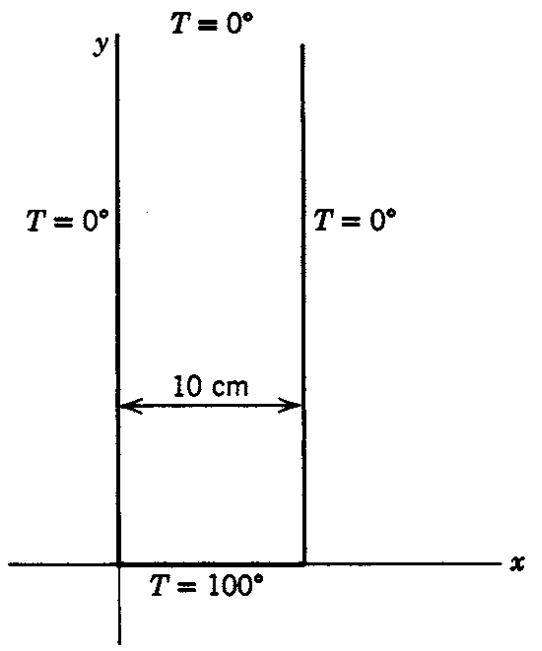
Our goal is to determine the steady–state temperature distribution \(T(x,y)\) in the plate.

1. Governing equation

In steady–state heat flow without internal heat sources, the temperature satisfies Laplace’s equation:

2. Separation of variables

We seek solutions of the form

Substituting into Laplace’s equation gives

Dividing by \(X(x)Y(y)\neq 0\) yields

Each term depends on a different variable, so each must equal a constant. We choose

which leads to the ODEs

3. Solving the \(X\)-equation

The general solution is

The side boundary conditions require

From \(X(0)=0\) we obtain \(B=0\), so

From \(X(a)=0\):

Thus the allowed eigenvalues are

4. Solving the \(Y\)-equation

For each eigenvalue \(k_n\), the equation

has the general solution

The temperature must remain finite and vanish as \(y\to\infty\):

This forces \(C = 0\), so

The separated solutions are therefore

5. Superposition and the base condition

By the linearity of Laplace’s equation, the full solution is a sum over all modes:

The base \(y=0\) is held at temperature \(T_0\):

which is the Fourier sine series of the constant function \(T_0\) on \((0,a)\).

Using the standard coefficient formula,

Thus

6. Final temperature distribution

Writing the odd indices as \(n = 2m+1\), the steady–state temperature distribution is

This satisfies all boundary conditions:

10.4Helmholtz Equation and the Infinite Spherical Well

Using the time dependence

the spatial wave function \(\psi(\mathbf{r})\) satisfies the time-independent Schrödinger equation.

10.4.1From Schrödinger to Helmholtz

The equation

simplifies to the Helmholtz equation

whenever \(V(\mathbf{r}) = V_{0}\) is constant, where

10.4.2Infinite Spherical Well

The potential for a 3D infinite spherical well is

Inside the well, \(V=0\), and thus

Boundary conditions:

This leads naturally to separation in spherical coordinates, producing Bessel functions in the radial equation and Legendre functions in the angular part.

10.4.3Separation in Spherical Coordinates: Three ODEs

In spherical coordinates \((r,\theta,\phi)\), the Laplacian is

We look for a fully separated solution of the form

Substituting into \(\nabla^2\psi + k^2\psi = 0\) and dividing by \(R\,\Theta\,\Phi\) gives

Group the radial and angular parts:

Since the first term depends only on \(r\) and the second only on \(\theta,\phi\), each must equal a constant. We choose a separation constant \(-\ell(\ell+1)\):

We now separate the angular equation further.

10.4.4Angular Equations: \(\Phi(\phi)\) and \(\Theta(\theta)\)

Start from

Multiply by \(\sin^2\theta\):

The first term depends only on \(\theta\), the second only on \(\phi\), so we separate again by setting each side equal to a constant, which we call \(-m^2\):

Thus we obtain two ODEs:

1. \(\phi\)-equation

   \begin{equation} \boxed{ \frac{d^2\Phi}{d\phi^2} + m^2 \Phi = 0. } \end{equation}

2. \(\theta\)-equation

   \begin{equation} \boxed{ \frac{1}{\sin\theta}\frac{d}{d\theta} \left(\sin\theta \frac{d\Theta}{d\theta}\right) + \left[\ell(\ell+1) - \frac{m^2}{\sin^2\theta}\right]\Theta(\theta) = 0. } \end{equation}

Solution of the \(\phi\)-equation.

The general solution is

Single-valuedness of \(\psi\) requires \(\Phi(\phi+2\pi) = \Phi(\phi)\), which implies

We usually choose the basis \(e^{im\phi}\), so we set

Solution of the \(\theta\)-equation.

With the substitution \(x = \cos\theta\), this equation becomes the associated Legendre equation. Its regular solutions are the associated Legendre functions:

with \(\ell = 0,1,2,\ldots\) and \(|m| \le \ell\).

Combining \(\Theta\) and \(\Phi\), the normalized angular functions are the spherical harmonics:

where \(N_{\ell m}\) is a normalization constant. The set \(\{Y_{\ell m}\}\) forms an orthonormal basis on the sphere.

Thus the angular part of the solution is completely determined:

10.4.5Radial Equation and Bessel Functions

The radial part of the separated solution satisfies

We now show how this can be solved in terms of ordinary Bessel functions of half–integer order.

Step 1. Non-dimensionalize the equation.

Introduce the dimensionless variable

so that

First expand the derivative in the radial equation:

Thus the equation becomes

Now rewrite everything in terms of \(x = kr\). Using \(r = x/k\),

and

Hence the radial equation becomes

Step 2. Reduce to the standard Bessel form.

The standard Bessel equation of order \(p\) is

Our equation has a \(2x \frac{dR}{dx}\) term instead of \(x \frac{dR}{dx}\), so we remove the extra factor by factoring out a square root. We set

and compute the derivatives:

Now substitute these into

Compute each term:

Add them together:

Group terms by powers of \(x\):

- Coefficient of \(x^{3/2}\): \(F'' + F\), - Coefficient of \(x^{1/2}\): \(-F' + 2F' = F'\), - Coefficient of \(x^{-1/2}\): \(\tfrac{3}{4}F - F - \ell(\ell+1)F = -\bigl(\ell(\ell+1) + \tfrac{1}{4}\bigr)F\).

Thus

Since \(x^{3/2}\neq 0\), the bracket must vanish:

Note that

so the equation becomes

which is precisely the Bessel equation of order

Step 3. General solution and return to \(R_\ell(r)\).

The general solution of the Bessel equation of order \(p\) is

so here

Recall that \(R(x) = x^{-1/2}F(x)\), hence

Returning to the original variable \(r\) with \(x = kr\), we obtain

Absorbing the overall factor \(1/\sqrt{k}\) into the constants and writing it in the conventional form,

Thus the radial equation for the infinite spherical well is solved in terms of ordinary Bessel functions of half–integer order.

where \(J_{p}\) and \(Y_{p}\) are the Bessel functions of the first and second kind.

Behavior near the origin. For small argument \(x\to 0\),

Thus for \(p=\ell+1/2>0\),

so the \(Y_{\ell+1/2}\) term diverges as \(r\to 0\).

Absorbing constants into a single coefficient, the physical radial solution inside the well is

10.4.6Boundary Condition and Energy Quantization

The infinite potential at \(r=a\) forces the wave function to vanish:

Since the spherical harmonic \(Y_{\ell m}(\theta,\phi)\) is never identically zero, this requires

Using the expression for \(R_\ell(r)\), this becomes

The prefactor is nonzero, so the boundary condition requires

Let \(\beta_{\ell n}\) denote the \(n\)-th positive zero of \(J_{\ell+1/2}(x)\):

Then

and the allowed energies are

The corresponding (unnormalized) stationary states are

with

Summary of the separation:

• The \(\phi\)-equation gives periodic solutions \(\Phi(\phi)=e^{im\phi}\).

• The \(\theta\)-equation gives associated Legendre functions \(P_\ell^{\,m}(\cos\theta)\).

• The radial equation gives Bessel functions of half-integer order \(J_{\ell+1/2}(kr)\).

Together these yield the full set of eigenfunctions \(\psi_{\ell m n}\) and quantized energies \(E_{\ell n}\).

10.5Where Partial Differential Equations Lead

This chapter is the destination the whole course has been heading toward. The two worked problems — the steady-state plate and the infinite spherical well — show the pattern: a partial differential equation is split by separation of variables into ordinary differential equations, each of which is one of the equations solved in the preceding chapters. Every tool built earlier reappears here doing its job.

• Every earlier chapter feeds in. Separation turns a PDE into ODEs (Chapter 8); at a regular singular point those ODEs are solved by series (Chapter 9), producing Legendre and Bessel functions; the boundary conditions are met by expanding in those orthogonal functions (Chapters 7 and 9); and in quantum problems the solutions are complex (Chapter 2) and the coordinate changes use the vector calculus of Chapters 5 and 6.

• The three classic equations. Laplace's equation (\(\nabla^2\psi=0\)) governs steady states — electrostatics, steady heat flow, incompressible flow. The diffusion equation adds a first time derivative; the wave equation a second. The same separation method handles all three.

• Geometry chooses the special functions. A rectangular box gives sines and cosines; a cylinder gives Bessel functions; a sphere gives Legendre functions and spherical harmonics. This is why the special functions of Chapter 9 are not optional — the shape of the problem selects them.

• Quantum mechanics. The infinite spherical well worked here is the template for the hydrogen atom: same separation, same angular solutions \(Y_{\ell m}\), with the radial equation changed by the Coulomb potential. The quantum numbers \((\ell, m, n)\) and the discrete energy levels come straight out of the boundary conditions, exactly as they did here.

• Boundary conditions quantize. The single most important lesson: a PDE has a continuum of separated solutions, but the boundary conditions select a discrete set. That is where standing-wave frequencies, atomic energy levels and normal modes all come from.

Summary Table

For the Interested Reader

Partial differential equations are a vast subject; this chapter has shown one method, separation of variables, applied to the cases where it works cleanly. That method covers a large fraction of the PDEs that arise in undergraduate physics, and it is the right place to start. Everything below is free.

Videos

3Blue1Brown's short films are the best picture of what a PDE says and why separating it into modes is natural. The second builds the heat equation — the same physics as the steady-state plate of this chapter — and then solves it exactly by the separation method used here:

Video

But what is a partial differential equation? — 3Blue1Brown

Watch on YouTube

Open video on YouTube

Video

Solving the heat equation — 3Blue1Brown

Watch on YouTube

Open video on YouTube

Websites

• Paul's Online Math Notes. Partial Differential Equations and Separation of Variables — worked heat- and wave-equation problems on an interval, with the Fourier-series step spelled out in full.