Chapter 3
Linear Algebra
3.1Linear Equations
Many problems in physics, engineering, and applied mathematics reduce to solving systems of linear equations: examples include Kirchhoff’s circuit laws, equilibrium conditions in mechanics, and eigenvalue problems in quantum mechanics.
A linear equation in the variables is an equation of the form
Each variable appears only to the first power: no products such as , and no nonlinear operations such as , , , etc.
Classify, as in the notes:
3.2System of Linear Equations
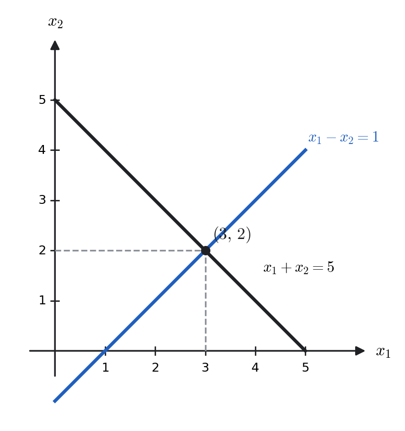
For two variables, each linear equation is a line. The solution(s) of a system are the intersection point(s) of those lines.
Solve
Solution.
Adding the two equations eliminates and gives , so ; substituting back gives . Hence
Geometrically each equation is a line, and the pair meets at a single point — the case of a unique solution.
3.2.1Matrix Form, and Augmented Matrix
A system of linear equations
can be written as , with coefficient matrix , unknown vector , and right-hand side . The augmented matrix is .
3.2.2Elementary Row Operations
Interchange two rows.
Multiply (or divide) a row by a nonzero constant.
Add a multiple of one row to another.
These do not change the solution set. That is the whole justification for row reduction: each operation is reversible, so the system you end up with has exactly the same solutions as the one you started with, while being far easier to read them off from.
3.2.3Row Echelon Form (REF) and Reduced Row Echelon Form (RREF)
A matrix is in row echelon form if:
all nonzero rows appear above any rows consisting entirely of zeros;
in each nonzero row, the first nonzero entry (called the leading entry or pivot) is to the right of the leading entry in the row above;
all entries below each leading entry are zero.
Important: In REF, pivots do not need to be .
A matrix is in reduced row echelon form if:
it is already in REF;
each leading entry is ;
each leading is the only nonzero entry in its column (including all entries above the pivot must be zero).
Examples of RREF:
Not RREF — Why?
Pivot in column 3 has nonzero entries above it, violating (iii).
of a matrix equals the number of pivots (nonzero rows) in its RREF.
3.3Gauss–Jordan Reduction
System:
This is RREF; unique solution.
infinitely many solutions. Let . Then
Last row is a contradiction. Hence
Let be the number of unknowns, the coefficient matrix, and the augmented matrix of a linear system.
If : Unique solution
If : Infinitely many solutions ( at least one free variable)
If : No solution (inconsistent system)
Your three quick cases:
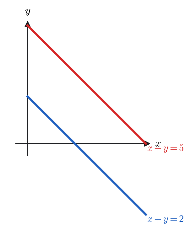
(a) Parallel lines No solution
Two distinct lines with the same slope never intersect.
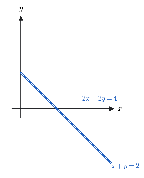
(b) Same line Infinitely many solutions
The equations represent the same geometric line.
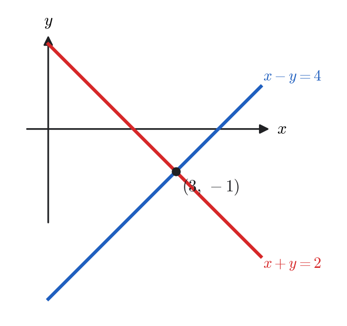
(c) Intersecting lines Unique solution
The lines meet at exactly one point.
3.4Determinants
Determinants provide a compact way of associating a scalar quantity with a square matrix. They are especially useful for testing invertibility and for solving systems of linear equations.
For
General Definition: Cofactor Expansion
Let be . Removing row and column gives the submatrix .
Expanding along row :
Properties of Determinants
Two identical rows/columns .
Swap two rows determinant changes sign.
Multiply a row by determinant multiplied by .
Add a multiple of one row to another determinant unchanged.
Triangular matrix determinant product of diagonal entries.
.
Compute the determinant:
Expand along the first row:
Compute each minor:
3.5Cramer's Rule
Let be an invertible matrix with . Consider the linear system
Let be the matrix obtained by replacing the -th column of with . Then each component of the unique solution is
Cramer's Rule is theoretically important, but computationally expensive for large systems. Practical numerical methods use row reduction instead of determinants.
Solve the system using Cramer’s Rule:
Coefficient matrix:
Replace columns:
Thus:
3.6Vectors
Definition and Notation
A vector is a mathematical object that has both magnitude and direction. In physics, vectors naturally describe quantities that not only have a size but also point in a specific direction. Examples include displacement, velocity, acceleration, force, momentum, and electric or magnetic fields.
Vector in 3D Space
For , the general definition becomes
In standard Cartesian coordinates we identify
so that in three-dimensional space, a vector is written in component form as
where are unit vectors along the axes, and are the components.
Magnitude of a Vector
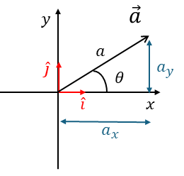
The magnitude (length) of is
If , then is a unit vector. Any nonzero vector can be turned into a unit vector by dividing by its length:
Multiplying a Vector by a Scalar
If is a real number (scalar), then
- If , the vector is stretched. - If , it is shrunk. - If , the direction is reversed.
Addition and Subtraction
For two vectors
we define
Geometrically, vector addition corresponds to placing the tail of at the head of (the parallelogram rule). Subtraction corresponds to adding .
Adding more than two vectors: If we have , then
In words: to add several vectors, add their components along each axis separately.
Geometric picture:
To add multiple vectors, place the tail of each vector at the head of the previous one (“tip-to-tail method”). The final vector goes from the start of the first to the tip of the last.
Subtracting a vector means adding its opposite. For example,
(3.50)
Dot Product (Scalar Product)
The dot product of and is defined by
where is the angle between and .
Component Formula
Write the vectors in components:
Now compute their dot product using distributivity:
Expanding term by term:
Using the orthonormality relations
all the cross terms vanish, leaving
Conclusion: The component definition
is equivalent to the geometric definition .
Let and . Then
Since the dot product is negative, the angle between the vectors is obtuse.
Let
Solution.
Step 2. Find the magnitudes.
Step 3. Use the formula.
Step 4. Solve for the angle.
Thus the angle between and is
Vectors in -Dimensional Space
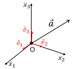
A vector in an -dimensional vector space is written as
where
are the components of the vector,
are the basis vectors of the space,
each points along the coordinate axis in the -th direction.
This expression is completely general: it defines a vector in any finite-dimensional vector space. In physics, however, we usually work in , which describes the three spatial directions.
Kronecker Delta and the Dot Product in Dimensions
Let be the standard orthonormal basis in . The inner product of two basis vectors is defined as
This property is written compactly using the Kronecker delta:
where
Dot Product in Dimensions
Let
The dot product is
Expanding:
Using :
Since is zero unless , this reduces to
Cross Product
For two vectors and in , the cross product is a new vector denoted by
Magnitude. The length of the cross product is defined by
where , , and is the angle between and .
Geometric interpretation.
is perpendicular to both and .
Its direction is given by the right-hand rule.
Its magnitude equals the area of the parallelogram spanned by and .
Component Formula for the Cross Product
Write the vectors in component form:
Then
Expanding term by term:
Now use the fundamental relations:
Substituting:
This is the component formula for the cross product. This is easiest to remember as a determinant, with the unit vectors in the first row:
Let and . Then
Levi-Civita Symbol and the Cross Product
In three dimensions, the cross product of the standard basis vectors is defined by
together with the antisymmetry property
These relations are compactly encoded by the Levi-Civita symbol:
where
Cross Product in 3D
Let
Then
Expanding:
Using the Levi-Civita relation:
Rearranging the sums:
Thus, the -th component of is
3.7Matrix Operations
3.7.1Matrix Equations
Two matrices are said to be equal if and only if they have the same size (same number of rows and columns) and each corresponding element is equal.
Two matrices and of the same size are equal if and only if all corresponding entries are equal. That is,
Consider the matrix equation
By equating corresponding elements, we find
3.7.2Multiplication of a Matrix by a Number
A scalar or can multiply a matrix . This operation means multiplying every entry of the matrix by .
Let be a matrix and let (or ). The scalar multiple of by is the matrix obtained by multiplying every entry of by :
Consider the vector
Multiplying by a scalar gives
Let
Then
For any matrix and scalar ,
In other words, scalar multiplication acts on each entry of the matrix.
Let be an matrix and a scalar. Then scaling every row of by scales the determinant by :
For the same as above, let . Then
Indeed,
3.7.3Matrix Addition
Two matrices of the same size can be added by adding their corresponding elements.
Let and be matrices of the *same size. Their sum is defined entry-wise:
For example,
Then
We can only add matrices if they have the same dimensions.
For matrices and of the same size,
Let
Then
Repeated addition of the same matrix corresponds to scalar multiplication:
3.7.4Matrix Multiplication
The product of two matrices is defined if and only if the number of columns of equals the number of rows of .
Let
Then the matrix product is the matrix whose entries are given by
Let
Since is and is , the product exists and is .
Note: cannot be computed because the dimensions do not match.
Let
Both products and can be computed.
Thus,
Associativity: .
Distributivity: .
Commutators and Anticommutators
For two square matrices and of the same size, the commutator is defined by
Consider
Rearranging gives
For two square matrices and of the same size, the anticommutator is defined by
Expanding
Let and be square matrices of the same size. Then
More generally, if are all square matrices of the same size, then
Let
First compute
Now compute
so
On the other hand,
Thus,
3.8Zero, Identity, and Transpose of Matrices
3.8.1Zero Matrix
A zero matrix, denoted , is a matrix in which every entry is zero. For any matrix of the same size,
A zero matrix:
3.8.2Identity Matrix
The identity matrix, denoted , is a square matrix with s on the main diagonal and s elsewhere. It acts as a multiplicative identity:
The identity matrix:
For
we have
3.8.3Transpose of a Matrix
The transpose of a matrix , denoted , is formed by interchanging rows and columns:
For any matrices and such that the product is defined,
From the definition,
Taking transpose:
On the other hand,
Thus,
Let
Compute
So
Meanwhile,
Hence
This result generalizes to multiple matrices:
3.8.4Inverse of a Matrix
Recall that the identity matrix satisfies
A square matrix is invertible (or nonsingular) if there exists a matrix such that
In this case, is called the inverse of .
If is an matrix with , then
where the adjugate matrix is the transpose of the cofactor matrix :
Each cofactor is given by
and is the submatrix formed by removing row and column of .
If
then
Let
Compute the cofactors:
- First row:
- Second row:
- Third row:
Thus the cofactor matrix is
Since
the inverse is
We write the system as
Solution.
Step 2. Cofactor matrix.
So
Step 3. Inverse matrix.
Step 4. Multiply by .
Compute components:
3.8.5Complex Conjugate of a Matrix
Let be a matrix with complex entries. The complex conjugate of , denoted or , is obtained by taking the complex conjugate of each entry:
3.8.6Hermitian Conjugate (Adjoint)
The Hermitian conjugate of a matrix , denoted , is defined as the transpose of its complex conjugate:
Equivalently,
If
3.8.7Special Matrices: Real vs Complex
It is useful to distinguish between real and complex matrices, because many important classes of matrices in the real case (such as symmetric and orthogonal) have natural generalizations in the complex case (Hermitian and unitary). This way, we can see clearly how the theory for real matrices extends to complex matrices.
| Real matrices | Complex matrices |
| – | (all entries real) |
| – | (Purely imaginary) |
| (Symmetric) | (Hermitian) |
| (Anti-symmetric) | (Anti-Hermitian) |
| (Orthogonal) | (Unitary) |
| – | (Normal) |
The correspondence is clear:
Let be a unitary matrix, i.e. .
Then
Thus, every unitary matrix is normal.
Also,
| Type | Definition | Example () |
| Real | ||
| Symmetric | ||
| Anti-symmetric | ||
| Orthogonal | ||
| Purely imaginary | ||
| Hermitian | ||
| Anti-Hermitian | ||
| Unitary | ||
| Normal |
3.8.8Functions of Matrices
We can extend the notion of a function of a number to a function of a matrix. In general, a function of a matrix is defined by the Taylor (Maclaurin) series expansion of , with the variable replaced by the matrix .
The Maclaurin series of a function is
Accordingly, we define
where is the identity matrix.
Let
a) Polynomial function of . First compute
Now consider
Using , higher powers reduce:
Thus
Therefore,
b) Exponential of using Maclaurin series. The exponential of a matrix is defined by
Using , higher powers alternate:
Thus
Recognizing the series expansions,
In general,
However, if (i.e., ), then
3.9Linear Combinations and Linear Functions
Let (or ) and let be scalars. Any vector of the form
is called a linear combination of and .
A function (or ) is linear if, for all scalars and vectors ,
Such functions are also called linear functionals.
A vector-valued function is linear if, for all scalars and vectors ,
Such functions are also called linear transformations or linear maps.
Is the exponential operator linear? Check:
Therefore, the exponential function is not linear.
Let be a function (operator) defined on a vector space . We say is a linear operator if, for all scalars and vectors ,
The derivative operator is linear because
Similarly, the integral operator
is linear since
3.10Matrix Operators and Linear Transformations
A linear transformation (or linear mapping) is a function
that maps vectors to vectors and satisfies, for all vectors and scalars ,
Equivalently, linear transformations preserve vector addition and scalar multiplication.
Linear Transformations in 2D
Consider the set of equations
where are constants.
For every point , these equations map it to a new point . This process is called a mapping or transformation of the plane. The matrix contains all the information about this transformation, and acts as a linear operator.
Since
the matrix is a linear operator.
Geometric Interpretation
Equations (3.215) can be interpreted in two ways:
The vector is mapped to a new vector in the same coordinate system.
Or, the coordinates of the same vector are expressed in a new coordinate system .
3.11Orthogonal Transformations
A real square matrix is called orthogonal if
Equivalently,
Thus, the columns (and rows) of an orthogonal matrix form an orthonormal set of vectors.
Conditions for a Orthogonal Matrix
Let
Then
For orthogonality, we require
Thus, the conditions are
Determinant Property
If is an orthogonal matrix, then
Since ,
But
so
3.12Rotation in 2D
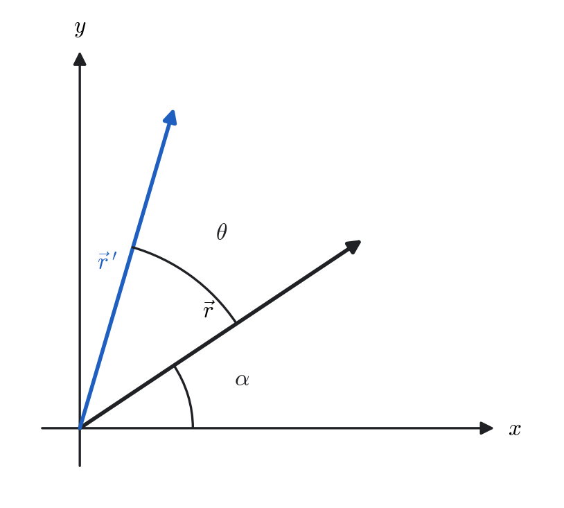
Active Rotation
Consider a vector
In polar form,
where and is the angle of the vector with the -axis.
Rotation of Coordinates
Suppose a vector in the plane is written in polar form as
where is the magnitude and is the angle with respect to the -axis.
After a counterclockwise rotation by an angle , the new vector becomes
Using the addition identities,
we substitute to obtain
Since and , this simplifies to
Resulting Coordinate Transformation
Thus, the rotated coordinates are
Matrix Form
This can be written in matrix form as
The matrix
is called the rotation matrix in 2D.
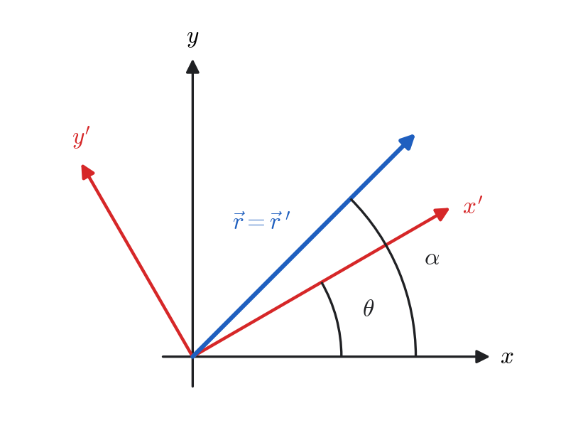
Passive Rotation
In a passive rotation, instead of rotating the vector, we rotate the coordinate system by , while keeping the vector fixed.
Equivalently, the components of the vector are expressed relative to the rotated axes . In this case, the relation between old and new coordinates is
3.13Rotations and Reflections in 3D
Rotations in three dimensions can be represented by special orthogonal matrices (). Reflections are also represented by orthogonal matrices, but with determinant .
Rotation about the -axis
A rotation by angle about the -axis is given by
Rotation about the -axis with reflection in the -plane
If we combine a rotation about with a reflection through the -plane, the matrix becomes
This is an orthogonal matrix with determinant .
Rotation about the -axis
A rotation by angle about the -axis is
Rotation about the -axis
A rotation by angle about the -axis is
General 3D Rotation
A general rotation in 3D can be expressed as a product of basic rotations:
Each rotation preserves vector length: .
The determinant distinguishes between a pure rotation () and a rotation combined with reflection ().
The product of orthogonal matrices is also orthogonal.
3.14Linear Independence
Vectors
A set of vectors is called linearly dependent if there exist scalars , not all zero, such that
A set of vectors is linearly independent if the only solution to
is the trivial solution:
Let
Then
so are linearly dependent.
However, the standard basis vectors are linearly independent since
Functions and Linear Dependence
Functions are called linearly dependent on an interval if there exist constants , not all zero, such that
If the only solution is , then the functions are linearly independent on .
Wronskian Test for Independence
Given functions that are -times differentiable, their Wronskian is defined as the determinant
If for at least one point (or on some subinterval) of the interval , then the functions are linearly independent on .
Consider the functions
The Wronskian is
Expanding the determinant:
Since (for ), the functions are linearly independent.
Linear independence is important because it tells us whether a set of functions (or vectors) provides genuinely new information. If functions are linearly dependent, then at least one of them can be expressed as a combination of the others, meaning it does not add anything new.
In differential equations, solutions are only useful if they are linearly independent. For example, the general solution of a second-order linear ODE requires two linearly independent solutions.
In Fourier series or orthogonal expansions, independence ensures that different basis functions represent different "directions" in function space.
In linear algebra, linear independence guarantees that a basis spans the space without redundancy, so every vector (or function) can be uniquely expressed as a combination of basis elements.
In short, linear independence is what allows us to build efficient and non-redundant representations of mathematical objects.
3.15Homogeneous Equations
General Form
A system of linear equations can be written as
If , the system is called a homogeneous system:
Basic Properties
Homogeneous equations are never inconsistent: the trivial solution always exists.
If , the system has only the trivial solution.
If , then there are infinitely many solutions.
Consider the system
In matrix form:
Here . Thus, the only solution is the trivial one: .
Consider the system
In matrix form:
Here . Thus, the system has infinitely many non-trivial solutions, e.g.
A homogeneous system of linear equations
where is an matrix, has non-trivial solutions () if and only if
Equivalently, the system has only the trivial solution when .
3.16Eigenvalues, Eigenvectors, and Matrix Diagonalization
From Linear Systems to Eigenvalue Problem
A general system of linear equations can be written as
A special case occurs when the vector on the right-hand side is proportional to , i.e.
Then
This is called the eigenvalue problem, where
is an eigenvalue,
is the corresponding eigenvector.
Rearranging,
This is a homogeneous system. For non-trivial solutions to exist, we require
which is called the characteristic equation.
The roots of this equation give the eigenvalues of . The corresponding eigenvectors are obtained by solving .
Find the eigenvalues and normalized eigenvectors of
Solution.
Step 1. Solve the characteristic equation.
Expanding,
Thus, the eigenvalues are
Step 2. Eigenvector for .
Solve
This gives . Take , then
Normalize:
Step 3. Eigenvector for .
Solve
This gives . Take , then
Normalize:
Orthogonality
Notice
Thus, and are orthogonal and normalized. This was not a coincidence: is symmetric, and the eigenvectors of a real symmetric matrix belonging to distinct eigenvalues are always orthogonal. That fact is why symmetric matrices are so prominent in physics — moments of inertia, stress tensors and quantum observables are all symmetric (or Hermitian), and each is guaranteed a set of perpendicular principal axes.
Matrix Diagonalization
If a matrix has linearly independent eigenvectors, then it can be diagonalized. That is, there exists a matrix such that
where is a diagonal matrix.
contains the eigenvalues of along its diagonal.
is the matrix whose columns are the eigenvectors of .
Explicitly,
From the previous example with
we found eigenvalues , , with normalized eigenvectors
Place them as the columns of , in the same order as the eigenvalues are listed in :
The order is not optional: swapping the columns of swaps the diagonal entries of . Since the eigenvectors are orthonormal, is orthogonal and , which makes the check easy:
Initially, in the standard -coordinate system, the matrix is not diagonal, so the action of mixes the two coordinates.
By finding eigenvectors, we identify new directions (the eigenvector directions) along which acts by simple stretching (scaling) without mixing.
Placing the eigenvectors as columns of gives a new coordinate system aligned with these eigenvector directions. In this new system:
and the matrix becomes diagonal.
Geometrically: is an orthogonal matrix (), so it represents a rotation of axes. This rotation “re-orients” the coordinate system so that the complicated mixing of in the basis becomes pure stretching along the new axes.
Degeneracy
If two or more eigenvalues of a matrix are equal, the eigenvalue is said to be degenerate. In this case, there may be more than one linearly independent eigenvector associated with the same eigenvalue.
Consider
The eigenvalues are
For : an eigenvector is
(3.291)For the degenerate eigenvalue : two linearly independent eigenvectors are
(3.292)
Thus, the eigenspace corresponding to is two-dimensional.
Degeneracy often arises in physics due to symmetries (e.g., rotational invariance). In such cases, the set of eigenvectors corresponding to a degenerate eigenvalue spans a subspace, and any linear combination of them is also an eigenvector.
3.16.5Application Diagonalization: Vibrations of a Linear Triatomic Molecule
Consider a linear triatomic molecule with three atoms connected by springs (see Figure 3.9). The outer atoms each have mass , and the central atom has mass . The spring constant is .
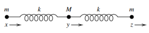
Let the displacements from equilibrium be denoted by for the left, middle, and right masses respectively. We are interested in finding the normal modes of vibration and the corresponding frequencies.
Potential Energy and Equations of Motion
The potential energy stored in the springs is
The equations of motion follow from Newton’s second law:
Normal Mode Ansatz
We seek normal mode solutions of the form
This leads to the eigenvalue problem
Let
The eigenvalues of this matrix are
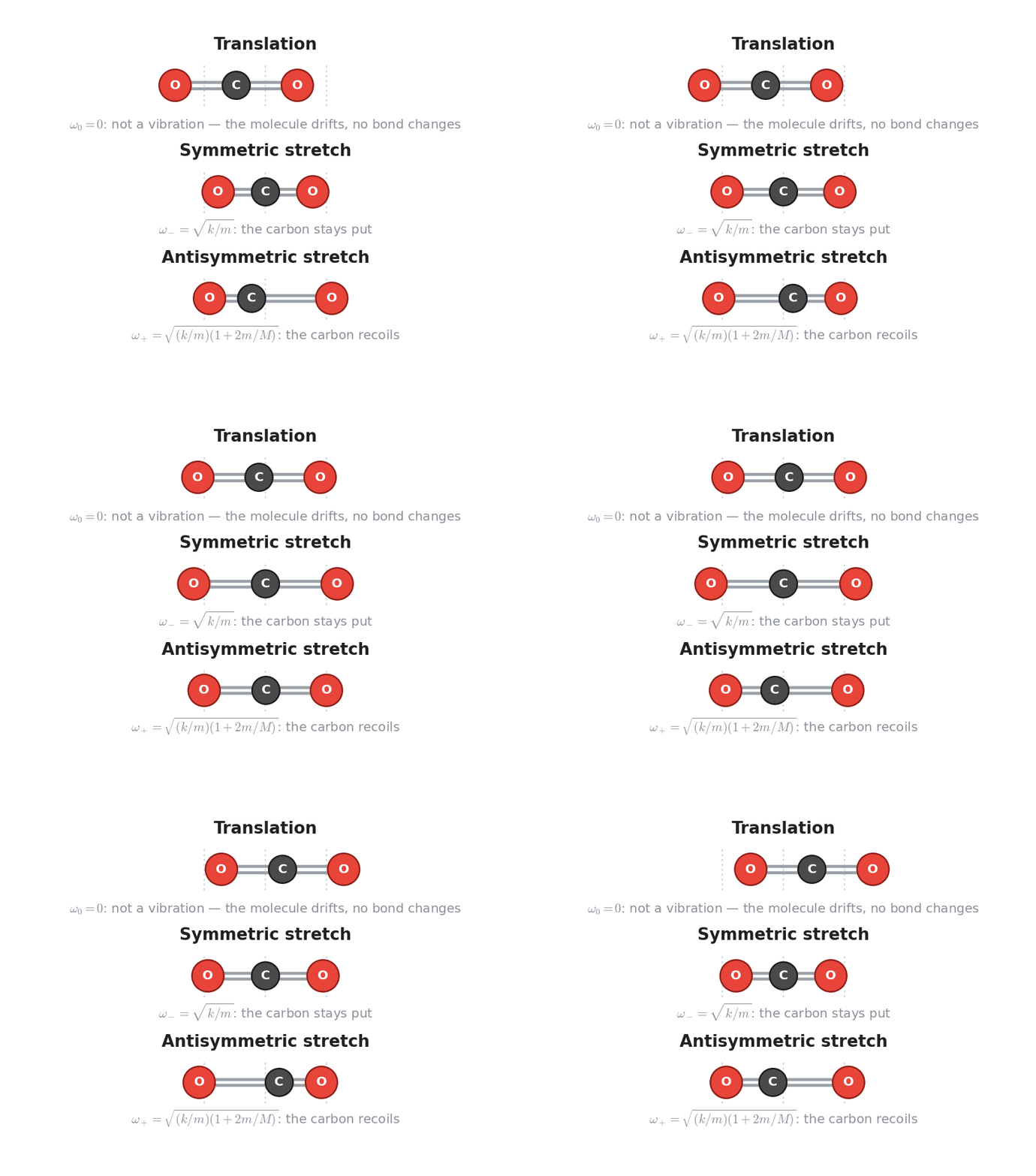
Modes by Symmetry
Translation (zero mode):
(3.302)Symmetric stretch:
(3.303)Antisymmetric stretch:
(3.304)(3.305)
Carbon dioxide is the standard example, since is linear and its outer atoms have equal mass: for oxygen and for carbon. Putting those numbers in gives , against the measured ratio for the two stretching bands of — close, for a model in which the molecule is three masses on two ideal springs. Water is not an example: is bent through about , and a bent molecule needs the two-dimensional problem.
3.17General Vector Spaces
Up to now, we have mostly thought of vectors as arrows in 2D or 3D space. However, the concept of a vector is much broader. Many mathematical objects (functions, polynomials, matrices, sequences) behave like vectors as long as they satisfy the same algebraic rules of addition and scalar multiplication. Such collections of objects are called vector spaces.
Definition of a Vector Space
A vector space over the real (or complex) numbers is a set of objects , called vectors, together with two operations:
Vector addition: for all ,
Scalar multiplication: for any scalar .
These operations must satisfy the following axioms:
Closure: .
Commutativity: .
Associativity: .
Zero vector: such that .
Additive inverse: For every , there exists such that .
Distributive properties:
(3.306)Associativity of scalar multiplication:
(3.307)Identity for scalar multiplication:
(3.308)
Examples of Vector Spaces
The set of all polynomials of degree ,
forms a vector space. The basis is
Any polynomial of degree can be written as a linear combination of these basis elements.
The set spans a vector space of functions. A basis is , or equivalently, .
The set of all matrices with real entries is a vector space. For example, the basis can be chosen as
3.18Bra–Ket Notation and Inner/Outer Products
Motivation
So far, we have written the dot product of two vectors as
In quantum mechanics and linear algebra, it is often convenient to use the Dirac notation, also called bra–ket notation, which provides a compact and powerful way to express inner and outer products.
Kets and Bras
A vector is written as a ket:
Its conjugate transpose is called a bra:
Inner Product (Dot Product)
The dot product (inner product) of two vectors is written as
Thus, the ordinary dot product
Outer Product
The outer product of two vectors is written as
This gives an matrix whose -th entry is .
Completeness Relation
For a complete set of orthonormal basis vectors ,
This is called the completeness relation.
In 3D space, the standard basis is
Then
Summary
= ket = column vector.
= bra = conjugate transpose (row vector).
= inner product (scalar).
= outer product (matrix).
Completeness: .
3.19Hilbert Spaces: Inner Product, Norm, and Orthogonality
Inner Product
For functions defined on an interval , the inner product is defined as
where is the complex conjugate of .
Norm
The norm (or length) of a function is
Orthogonality
Two functions are orthogonal if
Properties of Inner Product Spaces
An inner product space is a vector space with an additional inner product that satisfies:
Conjugate symmetry: .
Linearity in the second argument:
(3.324)Antilinearity in the first argument:
(3.325)Positive definiteness:
(3.326)
Hilbert Space
A Hilbert space is an inner product space that is also complete, meaning that all Cauchy sequences converge within the space. An important example is the space of square-integrable functions:
Functions in can be normalized so that
Orthonormal Bases
A set of functions is orthonormal if
Any function in the Hilbert space can be expanded as a linear combination:
For example, on the interval , the set
forms an orthogonal basis under the inner product
If the set is complete, then
Schwarz’s Inequality
For any two vectors (functions) in an inner product space,
This is a fundamental inequality that ensures consistency of the inner product structure.
3.20Gram–Schmidt Method of Orthonormalization
Motivation
Given a set of linearly independent vectors
we want to construct an orthonormal basis
The Gram–Schmidt procedure provides a systematic way to do this.
Procedure
Start with
(3.337)Subtract from its projection onto :
(3.338)Subtract from its projections onto both and :
(3.339)
At each step, we subtract projections to guarantee orthogonality, and then normalize to guarantee unit length.
Suppose we start with
Solution.
Step 1: Construct .
Step 2: Construct .
Compute
So
Normalize. Its squared length is , so and
Step 3: Construct .
Now subtract the projections onto both previous directions. The two inner products are
so
Its length is , giving
As a check, every pair is orthogonal and every vector has unit length:
Gram–Schmidt converts a linearly independent set of vectors into an orthonormal set.
In bra–ket notation: projections are written as .
Resulting vectors form an orthonormal basis: .
The construction is the reason an orthonormal basis can always be assumed to exist, which is used freely in quantum mechanics.
3.21Applications of Linear Algebra
Linear algebra earns its place in a physics course for a reason that is easy to miss while learning the mechanics of row reduction: most of physics is linear, or is studied by linearising it. Small oscillations about equilibrium, circuit networks, coupled differential equations, rigid-body rotation and all of quantum mechanics are linear problems, and a linear problem in variables is a matrix.
Normal modes. A system of coupled oscillators has equations of motion . Diagonalising finds coordinates in which the oscillators decouple; the eigenvalues are the squared frequencies and the eigenvectors are the patterns of motion. This is exactly the linear triatomic molecule worked through earlier in this chapter, and it recurs in Chapters 8 and 12.
Rigid-body rotation. The moment of inertia is a symmetric matrix, not a number. Its eigenvectors are the principal axes, about which a body spins without wobbling, and its eigenvalues are the principal moments.
Quantum mechanics. States are vectors, observables are Hermitian matrices, measured values are eigenvalues, and the bra–ket notation of the last section is the standard language. That measured quantities are real is precisely the statement that Hermitian matrices have real eigenvalues.
Circuits and networks. Kirchhoff's laws for a network with loops are simultaneous linear equations, solved by exactly the Gauss–Jordan row reduction of this chapter, or by Cramer's rule.
Coordinate changes. Rotations and reflections are orthogonal matrices. That they preserve lengths and angles is the single condition .
Notice how often the same two ideas did the work in this chapter. First, a matrix is not a table of numbers but a linear transformation, and the numbers only appear once a basis is chosen. Second, the natural basis for a problem is usually the eigenvector basis, in which the transformation stops mixing coordinates and simply stretches each axis. Almost every application above is an instance of choosing that better basis.
Summary Table
| Object | Definition | What it is for |
| Augmented matrix | Row reduce to solve . | |
| RREF | Pivots , zeros above and below | Reads off the solution set directly. |
| Determinant | invertible. | |
| Inverse | Solves . | |
| Dot product | Projection, work, orthogonality test. | |
| Cross product | Area, torque, angular momentum. | |
| Transpose | Symmetric if . | |
| Hermitian conjugate | Hermitian if ; real eigenvalues. | |
| Orthogonal matrix | Rotations and reflections; preserves length. | |
| Unitary matrix | The complex analogue; preserves probability. | |
| Eigenvalue problem | , | Normal modes, principal axes, observables. |
| Diagonalisation | , columns of are eigenvectors | Decouples the problem. |
| Linear independence | Only the trivial combination gives | Tested by , or the Wronskian for functions. |
For the Interested Reader
If the manipulations in this chapter felt mechanical — row reduce, expand a determinant, solve a characteristic polynomial — the resources below are worth your time, because they explain what those manipulations mean. Everything listed is free.
Videos
The strongest single recommendation in these notes is 3Blue1Brown's Essence of Linear Algebra. It builds the whole subject visually, from the one idea that a matrix is a transformation of space, and it explains the geometry that our algebra leaves implicit. If you watch only two things, watch these:
Vectors — Essence of Linear Algebra, Chapter 1
 Watch on YouTube
Linear transformations and matrices — Essence of Linear Algebra, Chapter 3
 Watch on YouTube
The series happens to run almost section-for-section alongside this chapter. Watch each episode when you reach the matching topic here:
Ch 1 — Vectors (our Vectors)
Ch 2 — Linear combinations, span and basis (Linear Independence)
Ch 3 — Linear transformations and matrices (Matrix Operators)
Ch 4 — Matrix multiplication as composition (Matrix Multiplication)
Ch 5 — Three-dimensional linear transformations (Rotations in 3D)
Ch 6 — The determinant (Determinants)
Ch 7 — Inverse matrices, column space and null space (Inverse of a Matrix; Homogeneous Equations)
Ch 8 — Nonsquare matrices as transformations between dimensions
Ch 9 — Dot products and duality (Dot Product)
Ch 10 — Cross products (Cross Product)
Ch 13 — Change of basis (Diagonalization)
Ch 14 — Eigenvectors and eigenvalues (Eigenvalues, Eigenvectors)
Ch 15 — A quick trick for computing eigenvalues (Eigenvalues)
Ch 16 — Abstract vector spaces (General Vector Spaces)
One more, from the same author's Differential Equations series rather than Essence of Linear Algebra, is the natural companion to our Functions of Matrices:
How (and why) to raise to the power of a matrix — 3Blue1Brown
 Watch on YouTube
Websites
Hefferon and Margalit–Rabinoff, Interactive Linear Algebra. A free online textbook with figures you can drag and manipulate in the browser — the same visual spirit as the videos, but where you do the moving. Good for the geometric meaning of span, independence and eigenspaces.
Paul's Online Math Notes — Linear Algebra. Notes and worked problems — the quick reference when you want more practice with a specific technique rather than a narrative.
A note on how to use these. Watch for the geometry first — what a determinant, an eigenvector or a change of basis does to space — and let that picture carry the algebra. In this course we mainly want to diagonalise a matrix to find normal modes, and to recognise when a physical problem is secretly a linear one; the eigenvalue episodes and the change-of-basis episode are the most directly useful for that.