Chapter 4

Partial Differentiation

4.1Introduction

In many physical problems, we encounter functions that depend on more than one variable, e.g.,

\begin{equation} f = f(x,y,z,\dots). \end{equation}

The partial derivative of $$f$$ with respect to $$x$$ means differentiating $$f$$ with respect to $$x$$ while treating all the other variables as constants. We denote this as

\begin{equation} \frac{\partial f}{\partial x}. \end{equation}

Definition - Partial Derivative

Let $f(x_1, x_2, \dots, x_n)$ be a function of several variables. The partial derivative of $$f$$ with respect to the variable $$x_i$$ is defined by

\begin{equation} \frac{\partial f}{\partial x_i} = \lim_{\Delta x_i \to 0} \frac{ f(x_1, \dots, x_i + \Delta x_i, \dots, x_n) - f(x_1, \dots, x_i, \dots, x_n) }{\Delta x_i}. \end{equation}

All other variables are held constant during the differentiation.

Notation

There are multiple notations for partial derivatives. For first-order:

\begin{equation} \frac{\partial f}{\partial x} = f_x. \end{equation}

For higher-order derivatives:

\begin{equation} \frac{\partial ^2 f}{\partial x^2} = f_{xx}, \qquad \frac{\partial ^2 f}{\partial x \partial y} = f_{xy}, \qquad \frac{\partial ^2 f}{\partial y^2} = f_{yy}. \end{equation}

Example - Partial Derivatives of a Multivariable Function

Let

\begin{equation} f(x,y) = x^3y - e^{xy}. \end{equation}

First-order partial derivatives:

\begin{equation} \frac{\partial f}{\partial x} = 3x^2y - y e^{xy}, \qquad \frac{\partial f}{\partial y} = x^3 - x e^{xy}. \end{equation}

Second-order partial derivatives:

\begin{equation} \frac{\partial ^2 f}{\partial x^2} = 6xy - y^2 e^{xy}, \qquad \frac{\partial ^2 f}{\partial y^2} = -x^2 e^{xy}. \end{equation}

\begin{equation} \frac{\partial ^2 f}{\partial x \partial y} = 3x^2 - e^{xy} - xy e^{xy}, \qquad \frac{\partial ^2 f}{\partial y \partial x} = 3x^2 - e^{xy} - xy e^{xy}. \end{equation}

Conclusion: Mixed partials agree:

\begin{equation} \frac{\partial ^2 f}{\partial x \partial y} = \frac{\partial ^2 f}{\partial y \partial x}, \end{equation}

(as long as $$f$$ is sufficiently smooth — Clairaut's Theorem).

Remark

For sufficiently smooth functions, the mixed derivatives are equal:

\begin{equation} \frac{\partial ^2 f}{\partial x \partial y} = \frac{\partial ^2 f}{\partial y \partial x}. \end{equation}

This is known as Clairaut’s theorem.

Example - Change of Variables and Partial Derivatives

Let

\begin{equation} z = x^2 - y^2, \qquad x = r\cos\theta,\quad y = r\sin\theta. \end{equation}

Then, using $$x^2 + y^2 = r^2$$ , we can rewrite $$z$$ in different but equivalent forms and compute $\frac{\partial z}{\partial r}$ while holding different variables constant.

1) Expressing $$z$$ in terms of $$r$$ and $\theta$ :

\begin{equation} z = r^2\cos^2\theta - r^2\sin^2\theta = r^2 \cos(2\theta). \end{equation}

Holding $\theta$ constant:

\begin{equation} \left(\frac{\partial z}{\partial r}\right)_{\theta} = 2r(\cos^2\theta - \sin^2\theta) = 2r\cos(2\theta). \end{equation}

2) Expressing $$z$$ in terms of $$x$$ and $$r$$ :

\begin{equation} z = 2x^2 - (x^2 + y^2) = 2x^2 - r^2. \end{equation}

Holding $$x$$ constant:

\begin{equation} \left(\frac{\partial z}{\partial r}\right)_{x} = -2r. \end{equation}

3) Expressing $$z$$ in terms of $$y$$ and $$r$$ :

\begin{equation} z = (x^2 + y^2) - 2y^2 = r^2 - 2y^2. \end{equation}

Holding $$y$$ constant:

\begin{equation} \left(\frac{\partial z}{\partial r}\right)_{y} = 2r. \end{equation}

Important: Each derivative is different because a different quantity is held fixed. Thus, we write:

\begin{equation} \left(\frac{\partial z}{\partial r}\right)_{\theta}, \qquad \left(\frac{\partial z}{\partial r}\right)_{x}, \qquad \left(\frac{\partial z}{\partial r}\right)_{y}, \end{equation}

to remove ambiguity in multivariable calculus.

4.2Applications in Thermodynamics

Partial derivatives play a central role in thermodynamics because most physical quantities depend on more than one variable. For example, temperature $$T$$ , pressure $$p$$ , volume $$V$$ , and entropy $$S$$ are related through equations of state and energy relations. To describe how one variable changes while others are held constant, we use partial derivatives with explicit subscripts.

For example, the temperature can be expressed as a function of pressure and volume,

\begin{equation} T = T(p,V), \end{equation}

or as a function of pressure and internal energy,

\begin{equation} T = T(p,U). \end{equation}

In these cases, we encounter derivatives such as

\begin{equation} \left(\frac{\partial T}{\partial p}\right)_V, \qquad \left(\frac{\partial T}{\partial p}\right)_U, \quad \dots \end{equation}

$\displaystyle \left(\frac{\partial T}{\partial p}\right)_V$ : how the temperature changes with pressure at constant volume. Physically this is a gas in a sealed rigid container: the volume cannot change, so heating the gas raises both its temperature and its pressure together. For an ideal gas $$pV = Nk_BT$$ gives $\left(\frac{\partial T}{\partial p}\right)_V = V/Nk_B$ directly.
$\displaystyle \left(\frac{\partial T}{\partial p}\right)_U$ : how the temperature changes with pressure at constant internal energy. This is the derivative relevant to the Joule free expansion, in which a gas expands into a vacuum inside rigid insulated walls: no heat enters and no work is done, so $$U$$ is unchanged. For an ideal gas $$U$$ depends on $$T$$ alone, so this derivative vanishes and the temperature does not change — a result that fails for a real gas, where it measures the intermolecular forces.

Remark

Constant $$U$$ is not the same as adiabatic. Adiabatic means no heat crosses the boundary, $\delta Q = 0$ ; for a reversible process that is constant entropy, $$S$$ . A gas compressed adiabatically does have work done on it, so its internal energy rises. The free expansion above happens to be both adiabatic and at constant $$U$$ only because no work is done either.

Remark

The subscript indicates which variables are kept constant during differentiation. For example:

\begin{equation} \left(\frac{\partial T}{\partial p}\right)_V \quad \text{means ``change in $T$ with respect to $p$ while keeping $V$ fixed.''} \end{equation}

This removes ambiguity and prevents misinterpretation of derivatives.

Example - Physics: the thermodynamic cyclic relation

A gas has an equation of state relating $$p$$ , $$V$$ and $$T$$ , such as $$pV = Nk_BT$$ , so that any one of the three is determined by the other two. Show that

\begin{equation} \left(\frac{\partial p}{\partial V}\right)_T \left(\frac{\partial V}{\partial T}\right)_p \left(\frac{\partial T}{\partial p}\right)_V = -1 . \label{eq:cyclic_relation} \end{equation}

Solution.

The result is surprising at first sight: one might expect the three factors to cancel to $$+1$$ , as they would if the symbols were ordinary fractions. They do not, and the minus sign is the point.

Regard $$T$$ as a function of $$p$$ and $$V$$ and write its total differential:

\begin{equation} dT = \left(\frac{\partial T}{\partial p}\right)_V dp + \left(\frac{\partial T}{\partial V}\right)_p dV . \end{equation}

Now specialise to a process at constant temperature, so $$dT = 0$$ :

\begin{equation} 0 = \left(\frac{\partial T}{\partial p}\right)_V dp + \left(\frac{\partial T}{\partial V}\right)_p dV . \end{equation}

Dividing by $$dV$$ at fixed $$T$$ and solving for the ratio gives

\begin{equation} \left(\frac{\partial p}{\partial V}\right)_T = - \frac{\left(\frac{\partial T}{\partial V}\right)_p}{\left(\frac{\partial T}{\partial p}\right)_V}. \end{equation}

Substitute this into the left-hand side of $\eqref{eq:cyclic_relation}$ . The middle factor may be inverted, because $\left(\frac{\partial V}{\partial T}\right)_p$ and $\left(\frac{\partial T}{\partial V}\right)_p$ hold the same variable $$p$$ fixed and so are genuine reciprocals:

\begin{equation} \left(\frac{\partial p}{\partial V}\right)_T \left(\frac{\partial V}{\partial T}\right)_p \left(\frac{\partial T}{\partial p}\right)_V = - \frac{\left(\frac{\partial T}{\partial V}\right)_p}{\left(\frac{\partial T}{\partial p}\right)_V} \cdot \frac{1}{\left(\frac{\partial T}{\partial V}\right)_p} \cdot \left(\frac{\partial T}{\partial p}\right)_V = -1 . \end{equation}

As a check, use the ideal gas law $$pV = Nk_BT$$ directly:

\begin{equation} \left(\frac{\partial p}{\partial V}\right)_T = -\frac{Nk_BT}{V^2}, \qquad \left(\frac{\partial V}{\partial T}\right)_p = \frac{Nk_B}{p}, \qquad \left(\frac{\partial T}{\partial p}\right)_V = \frac{V}{Nk_B}, \end{equation}

whose product is $-\dfrac{Nk_BT}{V\,p} = -1$ , since $$pV = Nk_BT$$ .

The minus sign has a physical reading. Raise the pressure at fixed volume and the temperature rises; raise the temperature at fixed pressure and the volume rises; so increasing the volume at fixed temperature must lower the pressure. Two increases and one decrease give the negative sign. This relation is used constantly in thermodynamics to trade an unmeasurable derivative for two measurable ones.

4.3Power Series in Two Variables

Just as a function of a single variable can be expressed as a power series expansion, functions of two variables can also be expanded into a series about a point $$(a,b)$$ .

Example - Series Expansion of

\sin(x)\cos(y)

Use the power series

\begin{equation} \sin(x) = x - \frac{x^3}{3!} + \frac{x^5}{5!} - \cdots, \qquad \cos(y) = 1 - \frac{y^2}{2!} + \frac{y^4}{4!} - \cdots. \end{equation}

Multiply the expansions:

\begin{equation} \sin(x)\cos(y) = \left(x - \frac{x^3}{3!} + \cdots\right) \left(1 - \frac{y^2}{2!} + \cdots\right). \end{equation}

Collecting lowest-order terms:

\begin{equation} = x - \frac{x^3}{3!} - \frac{x y^2}{2!} + \cdots \end{equation}

Thus, the (truncated) power-series expansion is:

\begin{equation} \boxed{\sin(x)\cos(y) = x - \frac{x^3}{6} - \frac{xy^2}{2} + \cdots} \end{equation}

Example - Series Expansion of

\ln(1+x-y)

Start with the known expansion (for $$|z|<1$$ ):

\begin{equation} \ln(1+z) = z - \frac{z^2}{2} + \frac{z^3}{3} - \cdots. \end{equation}

Let $$z = x - y$$ :

\begin{equation} \ln(1+x-y) = (x-y) - \frac{(x-y)^2}{2} + \frac{(x-y)^3}{3} - \cdots. \end{equation}

Expand:

\begin{equation} = (x-y) - \frac{x^2 - 2xy + y^2}{2} + \frac{x^3 - 3x^2y + 3xy^2 - y^3}{3} - \cdots \end{equation}

Simplify:

\begin{equation} \boxed{ \ln(1+x-y) = x - y - \frac{x^2}{2} + xy - \frac{y^2}{2} + \frac{x^3}{3} - x^2y + xy^2 - \frac{y^3}{3} + \cdots } \end{equation}

General Expansion

In general, a sufficiently smooth function $$f(x,y)$$ can be expanded in a power series about a point $$(a,b)$$ as

\begin{equation} f(x,y) = \sum_{n=0}^{\infty} \frac{1}{n!} \left((x-a)\frac{\partial}{\partial X} + (y-b)\frac{\partial}{\partial Y}\right)^n \left.f(X,Y)\right|_{(a,b)}. \label{eq:taylor_two_var} \end{equation}

This is the multivariable Taylor series expansion. The operator in brackets is raised to the $$n$$ th power before acting on $$f$$ , so at order $$n$$ it produces every mixed derivative of total order $$n$$ , each weighted by a binomial coefficient. Writing out $$n=2$$ gives the familiar three terms in $$x^2$$ , $$xy$$ and $$y^2$$ used below.

Taylor Expansion Approach

Instead of multiplying series, we can also compute the expansion of

\begin{equation} f(x,y) = \sin(x)\cos(y) \end{equation}

directly using the two-variable Taylor series about $$(0,0)$$ :

\begin{equation} \begin{aligned} f(x,y) &= f(0,0) + \left.\frac{\partial f}{\partial X}\right|_{(0,0)} x + \left.\frac{\partial f}{\partial Y}\right|_{(0,0)} y \\[6pt] &\quad + \frac{1}{2!}\Bigg[ \left.\frac{\partial^{2} f}{\partial X^{2}}\right|_{(0,0)} x^2 + 2 \left.\frac{\partial^{2} f}{\partial X\,\partial Y}\right|_{(0,0)} xy + \left.\frac{\partial^{2} f}{\partial Y^{2}}\right|_{(0,0)} y^2 \Bigg] + \cdots \end{aligned} \end{equation}

Step 1. Zeroth order

\begin{equation} f(0,0) = \sin(0)\cos(0) = 0. \end{equation}

Step 2. First order

\begin{equation} \frac{\partial f}{\partial X} = \cos(X)\cos(Y), \quad \left.\frac{\partial f}{\partial X}\right|_{(0,0)} = 1, \end{equation}

\begin{equation} \frac{\partial f}{\partial Y} = -\sin(X)\sin(Y), \quad \left.\frac{\partial f}{\partial Y}\right|_{(0,0)} = 0. \end{equation}

So the linear contribution is $$x$$ .

Step 3. Second order

At $$(0,0)$$ , all second derivatives vanish, so there is no quadratic contribution.

Step 4. Third order

At third order the bracket in $\eqref{eq:taylor_two_var}$ produces four terms, not one:

\begin{equation} \frac{1}{3!}\Bigg[ \left.\frac{\partial^{3} f}{\partial X^{3}}\right|_{(0,0)} x^3 + 3\left.\frac{\partial ^3 f}{\partial X^2 \partial Y}\right|_{(0,0)} x^2 y + 3\left.\frac{\partial ^3 f}{\partial X \partial Y^2}\right|_{(0,0)} x y^2 + \left.\frac{\partial^{3} f}{\partial Y^{3}}\right|_{(0,0)} y^3 \Bigg]. \end{equation}

Evaluating each at the origin, where $\sin$ vanishes and $\cos$ equals one:

\begin{equation} \frac{\partial^{3} f}{\partial X^{3}} = -\cos X\cos Y \ \to\ -1, \qquad \frac{\partial ^3 f}{\partial X \partial Y^2} = -\cos X\cos Y \ \to\ -1, \end{equation}

\begin{equation} \frac{\partial ^3 f}{\partial X^2 \partial Y} = \sin X\sin Y \ \to\ 0, \qquad \frac{\partial^{3} f}{\partial Y^{3}} = \sin X\sin Y \ \to\ 0 . \end{equation}

So the third-order contribution is

\begin{equation} \frac{1}{6}\Big[-x^3 + 3(-1)xy^2\Big] = -\frac{x^3}{6} - \frac{xy^2}{2}. \end{equation}

Result

Collecting terms:

\begin{equation} \sin(x)\cos(y) = x - \frac{x^3}{6} - \frac{xy^2}{2} + \cdots \end{equation}

Remark

This matches the result obtained earlier by multiplying the single-variable series, including the $$xy^2$$ term. That term is easy to lose: it comes from the mixed derivative $\frac{\partial ^3 f}{\partial X \partial Y^2}$ , not from differentiating three times in $$x$$ . When using the multivariable Taylor series, every mixed derivative of the given total order must be included, each with its binomial coefficient.

4.4Total Differentials

Review: One Variable

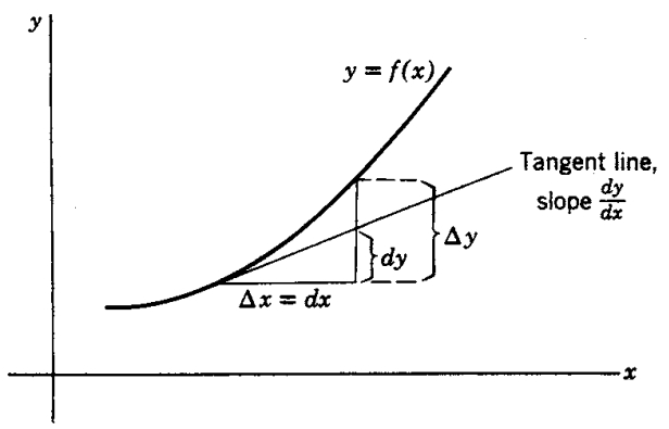
Illustration of the differential: for a small change dx, the corresponding change in y is approximated by dy = y' dx. — Figure 4.1. Illustration of the differential: for a small change $$dx$$ , the corresponding change in $$y$$ is approximated by $$dy = y' dx$$ .

If $$y = f(x)$$ , then

\begin{equation} y' = \frac{d y}{d x} = \frac{d f(x)}{d x}. \end{equation}

By definition,

\begin{equation} \frac{d y}{d x} = \lim_{\Delta x \to 0} \frac{\Delta y}{\Delta x}. \end{equation}

Hence, for small $\Delta x$ ,

\begin{equation} dx = \Delta x, \qquad dy = y' \, dx. \end{equation}

Two Variables

If $$f = f(x,y)$$ , then the total differential is

\begin{equation} df = \frac{\partial f}{\partial x} dx + \frac{\partial f}{\partial y} dy. \end{equation}

General Case

For a function of many variables,

\begin{equation} f = f(x,y,z,\dots), \end{equation}

the total differential is

\begin{equation} df = \frac{\partial f}{\partial x} dx + \frac{\partial f}{\partial y} dy + \frac{\partial f}{\partial z} dz + \cdots \end{equation}

Remark

The total differential expresses the approximate change in $$f$$ resulting from small changes in its independent variables.

4.5Chain Rule: Differentiating a Function of a Function

The chain rule extends naturally to functions of functions. If a variable depends on another, which in turn depends on a third, we can differentiate by following the chain of dependencies.

Theorem - Chain Rule for Composite Functions

If $$y = y(u)$$ and $$u = u(x)$$ , then the derivative of $$y$$ with respect to $$x$$ is

\begin{equation} \boxed{\frac{d y}{d x} = \frac{d y}{d u}\,\frac{d u}{d x}}. \end{equation}

More generally, if

\begin{equation} u = u(x,y), \qquad x = x(t), \qquad y = y(t), \end{equation}

then

\begin{equation} \boxed{\frac{d u}{d t} = \frac{\partial u}{\partial x}\,\frac{d x}{d t} + \frac{\partial u}{\partial y}\,\frac{d y}{d t}}. \end{equation}

For functions depending on multiple variables,

\begin{equation} \boxed{ \frac{d u}{d t} = \frac{\partial u}{\partial x}\,\frac{d x}{d t} + \frac{\partial u}{\partial y}\,\frac{d y}{d t} + \frac{\partial u}{\partial z}\,\frac{d z}{d t} + \cdots } \end{equation}

where the sum includes a term for each independent variable.

Example

Let

\begin{equation} y = \ln(u), \qquad u = \sin(v), \qquad v = 2x. \end{equation}

Find $\frac{d y}{d x}$ .

Solution.

\begin{equation} \frac{d y}{d x} = \frac{d y}{d u}\,\frac{d u}{d v}\,\frac{d v}{d x}. \end{equation}

Compute the derivatives step by step:

\begin{equation} \frac{d y}{d u} = \frac{1}{u}, \qquad \frac{d u}{d v} = \cos(v), \qquad \frac{d v}{d x} = 2. \end{equation}

Thus,

\begin{equation} \frac{d y}{d x} = \frac{1}{u}\cos(v)\cdot 2 = \frac{2\cos(v)}{u}. \end{equation}

Since $u=\sin(v)$ ,

\begin{equation} \boxed{\frac{d y}{d x} = \frac{2\cos(v)}{\sin(v)} = 2\cot(v) = 2\cot(2x).} \end{equation}

Example

Let

\begin{equation} z = x y, \qquad x = 2t^2, \qquad y = \sin(t). \end{equation}

Find $\frac{d z}{d t}$ .

Solution.

\begin{equation} \frac{d z}{d t} = \frac{\partial z}{\partial x}\frac{d x}{d t} + \frac{\partial z}{\partial y}\frac{d y}{d t}. \end{equation}

Since

\begin{equation} \frac{\partial z}{\partial x} = y, \qquad \frac{\partial z}{\partial y} = x, \end{equation}

we get

\begin{equation} \frac{d z}{d t} = y\,\frac{d x}{d t} + x\,\frac{d y}{d t}. \end{equation}

Now compute the derivatives:

\begin{equation} \frac{d x}{d t} = 4t, \qquad \frac{d y}{d t} = \cos(t). \end{equation}

Therefore,

\begin{equation} \frac{d z}{d t} = \sin(t)(4t) + (2t^2)\cos(t). \end{equation}

\begin{equation} \boxed{\frac{d z}{d t} = 4t\sin(t) + 2t^2\cos(t).} \end{equation}

Remark

The chain rule allows us to differentiate composite functions systematically, even when variables are nested or interdependent.

4.6Implicit Differentiation

Often, functions are defined implicitly rather than explicitly. For example, if $$x$$ and $$t$$ are related by

\begin{equation} x + e^x = t, \end{equation}

then $$x$$ is an implicit function of $$t$$ .

First Derivative

Differentiate both sides of

\begin{equation} x + e^x = t \end{equation}

with respect to $$t$$ :

\begin{equation} \frac{d x}{d t} + e^x \frac{d x}{d t} = 1. \end{equation}

Thus,

\begin{equation} \frac{d x}{d t} = \frac{1}{1+e^x}. \end{equation}

Second Derivative

From the expression for $\frac{d x}{d t}$ , we differentiate again:

\begin{equation} \frac{d^{2} x}{d t^{2}} = \frac{d}{d t}\!\left[(1+e^x)^{-1}\right]. \end{equation}

Apply the chain rule:

\begin{equation} \frac{d^{2} x}{d t^{2}} = -(1+e^x)^{-2}\cdot e^x \frac{d x}{d t}. \end{equation}

Now substitute $\frac{d x}{d t} = \dfrac{1}{1+e^x}$ :

\begin{equation} \frac{d^{2} x}{d t^{2}} = -\frac{e^x}{(1+e^x)^3}. \end{equation}

Example

Find the equation of the tangent line to the curve

\begin{equation} x^3 - 3y^3 + xy + 21 = 0 \end{equation}

at the point $$(1,2)$$ .

Solution.

First check that the point actually lies on the curve, since everything below depends on it:

\begin{equation} 1^3 - 3(2)^3 + (1)(2) + 21 = 1 - 24 + 2 + 21 = 0 . \checkmark \end{equation}

Now differentiate implicitly with respect to $$x$$ , remembering that $$y$$ is a function of $$x$$ , so $$y^3$$ and $$xy$$ need the chain and product rules:

\begin{equation} 3x^2 - 9y^2\,\frac{d y}{d x} + y + x\,\frac{d y}{d x} = 0. \end{equation}

Group the $\frac{d y}{d x}$ terms:

\begin{equation} (x - 9y^2)\frac{d y}{d x} = -(3x^2 + y). \end{equation}

Solve for slope:

\begin{equation} \frac{d y}{d x} = \frac{-(3x^2 + y)}{x - 9y^2}. \end{equation}

At the point $$(1,2)$$ :

\begin{equation} \frac{d y}{d x}\Big|_{(1,2)} = \frac{-(3(1)^2 + 2)}{1 - 9(2^2)} = \frac{-5}{-35} = \frac{1}{7}. \end{equation}

The tangent line with slope $m = \frac{1}{7}$ at $$(1,2)$$ :

\begin{equation} y - 2 = \frac{1}{7}(x - 1). \end{equation}

Simplifying:

\begin{equation} \boxed{x - 7y + 13 = 0.} \end{equation}

Remark

Implicit differentiation allows us to compute derivatives (and tangent lines) for curves not expressed explicitly as $$y=f(x)$$ .

4.7More on Chain Rule

Theorem - General Chain Rule

Suppose

\begin{equation} u = u(x,y,z), \qquad x = x(s,t), \quad y = y(s,t), \quad z = z(s,t). \end{equation}

Then the chain rule gives

\begin{equation} \boxed{ \frac{\partial u}{\partial s} = \frac{\partial u}{\partial x}\frac{\partial x}{\partial s} + \frac{\partial u}{\partial y}\frac{\partial y}{\partial s} + \frac{\partial u}{\partial z}\frac{\partial z}{\partial s}} \end{equation}

\begin{equation} \boxed{ \frac{\partial u}{\partial t} = \frac{\partial u}{\partial x}\frac{\partial x}{\partial t} + \frac{\partial u}{\partial y}\frac{\partial y}{\partial t} + \frac{\partial u}{\partial z}\frac{\partial z}{\partial t}} \end{equation}

Write the total differential of $$u=u(x,y,z)$$ :

\begin{equation} du = \frac{\partial u}{\partial x}\,dx + \frac{\partial u}{\partial y}\,dy + \frac{\partial u}{\partial z}\,dz. \end{equation}

Since $x=x(s,t),\; y=y(s,t),\; z=z(s,t)$ , their differentials are

\begin{equation} dx = \frac{\partial x}{\partial s}\,ds + \frac{\partial x}{\partial t}\,dt,\qquad dy = \frac{\partial y}{\partial s}\,ds + \frac{\partial y}{\partial t}\,dt,\qquad dz = \frac{\partial z}{\partial s}\,ds + \frac{\partial z}{\partial t}\,dt. \end{equation}

Substitute into $$du$$ and collect coefficients of $$ds$$ and $$dt$$ :

\begin{equation} \begin{aligned} du &= \Big(\frac{\partial u}{\partial x}\frac{\partial x}{\partial s} + \frac{\partial u}{\partial y}\frac{\partial y}{\partial s} + \frac{\partial u}{\partial z}\frac{\partial z}{\partial s}\Big)\,ds \\ &\quad + \Big(\frac{\partial u}{\partial x}\frac{\partial x}{\partial t} + \frac{\partial u}{\partial y}\frac{\partial y}{\partial t} + \frac{\partial u}{\partial z}\frac{\partial z}{\partial t}\Big)\,dt. \end{aligned} \end{equation}

By the definition of partial derivatives of $$u$$ as a function of $$(s,t)$$ ,

\begin{equation} \frac{\partial u}{\partial s} = \frac{\partial u}{\partial x}\frac{\partial x}{\partial s} + \frac{\partial u}{\partial y}\frac{\partial y}{\partial s} + \frac{\partial u}{\partial z}\frac{\partial z}{\partial s},\qquad \frac{\partial u}{\partial t} = \frac{\partial u}{\partial x}\frac{\partial x}{\partial t} + \frac{\partial u}{\partial y}\frac{\partial y}{\partial t} + \frac{\partial u}{\partial z}\frac{\partial z}{\partial t}. \end{equation}

Writing these two identities together in matrix form gives

\begin{equation} \begin{pmatrix} \frac{\partial u}{\partial s} & \frac{\partial u}{\partial t} \end{pmatrix} = \begin{pmatrix} \frac{\partial u}{\partial x} & \frac{\partial u}{\partial y} & \frac{\partial u}{\partial z} \end{pmatrix} \begin{pmatrix} \frac{\partial x}{\partial s} & \frac{\partial x}{\partial t} \\[6pt] \frac{\partial y}{\partial s} & \frac{\partial y}{\partial t} \\[6pt] \frac{\partial z}{\partial s} & \frac{\partial z}{\partial t} \end{pmatrix}, \end{equation}

which is the desired matrix chain rule. Check the shapes: a $1\times3$ row times a $3\times2$ matrix gives a $1\times2$ row, one entry for each of $$s$$ and $$t$$ . The middle matrix is the Jacobian of the change of variables, and the chain rule is just matrix multiplication by it.

Example

Let

\begin{equation} z = xy, \qquad x = \sin(s+t), \qquad y = s - t. \end{equation}

We want to compute $\frac{\partial z}{\partial s}$ and $\frac{\partial z}{\partial t}$ .

Solution.

Step 1. Apply the Chain Rule

\begin{equation} \frac{\partial z}{\partial s} = \frac{\partial z}{\partial x}\frac{\partial x}{\partial s} + \frac{\partial z}{\partial y}\frac{\partial y}{\partial s}, \qquad \frac{\partial z}{\partial t} = \frac{\partial z}{\partial x}\frac{\partial x}{\partial t} + \frac{\partial z}{\partial y}\frac{\partial y}{\partial t}. \end{equation}

Step 2. Compute partial derivatives of $$z$$

Since $$z = xy$$ ,

\begin{equation} \frac{\partial z}{\partial x} = y, \qquad \frac{\partial z}{\partial y} = x. \end{equation}

Step 3. Compute derivatives of $$x$$ and $$y$$

\begin{equation} x = \sin(s+t) \Rightarrow \frac{\partial x}{\partial s} = \cos(s+t), \quad \frac{\partial x}{\partial t} = \cos(s+t), \end{equation}

\begin{equation} y = s - t \Rightarrow \frac{\partial y}{\partial s} = 1, \quad \frac{\partial y}{\partial t} = -1. \end{equation}

Step 4. Substitute and simplify

\begin{equation} \frac{\partial z}{\partial s} = y\cos(s+t) + x, \qquad \frac{\partial z}{\partial t} = y\cos(s+t) - x. \end{equation}

\begin{equation} \boxed{ \frac{\partial z}{\partial s} = (s - t)\cos(s+t) + \sin(s+t), \qquad \frac{\partial z}{\partial t} = (s - t)\cos(s+t) - \sin(s+t) } \end{equation}

Example

For

\begin{equation} z=x-y,\qquad x^2+y^2=t^2,\qquad x\sin t=ye^y, \end{equation}

find $\frac{d z}{d t}=?$

Solution.

Step 1. Differentiate the constraints.

\begin{equation} 2x\,dx+2y\,dy=2t\,dt, \qquad \sin t\,dx+x\cos t\,dt=(y+1)e^y\,dy. \end{equation}

Step 2. Rearrange to a linear system for $$dx,dy$$ .

\begin{equation} x\,dx+y\,dy=t\,dt, \qquad \sin t\,dx-(y+1)e^y\,dy=-x\cos t\,dt. \end{equation}

Step 3. Solve for $$dx$$ (and similarly $$dy$$ ) by determinants.

\begin{equation} dx =\frac{ \begin{vmatrix} t\,dt & y\\[4pt] - x\cos t\,dt & -(y+1)e^y \end{vmatrix} }{ \begin{vmatrix} x & y\\[4pt] \sin t & -(y+1)e^y \end{vmatrix} } =\frac{-t(y+1)e^y + xy\cos t}{-x(y+1)e^y - y\sin t}\,dt. \end{equation}

Equivalently,

\begin{equation} \frac{dx}{dt} =\frac{t(y+1)e^y - xy\cos t}{x(y+1)e^y + y\sin t}. \end{equation}

A parallel computation gives

\begin{equation} dy =\frac{ \begin{vmatrix} x & t\,dt \\[4pt] \sin t & -x\cos t\,dt \end{vmatrix} }{ \begin{vmatrix} x & y \\[4pt] \sin t & -(y+1)e^y \end{vmatrix} } =\frac{-x^{2}\cos t - t\sin t}{-x(y+1)e^y - y\sin t}\,dt. \end{equation}

Equivalently,

\begin{equation} \frac{dy}{dt} =\frac{x^{2}\cos t + t\sin t}{x(y+1)e^y + y\sin t}. \end{equation}

Since $$z = x - y$$ , we have

\begin{equation} \frac{dz}{dt}=\frac{dx}{dt}-\frac{dy}{dt}. \end{equation}

Example

Find $\frac{\partial z}{\partial s}$ and $\frac{\partial z}{\partial t}$ given

\begin{equation} z = x^2 + xy, \qquad x^2 + y^3 = st + 5, \qquad x^3 - y^2 = s^2 + t^2. \end{equation}

Solution.

Step 1. Differential of $$z$$

We compute

\begin{equation} dz = \frac{\partial z}{\partial x} dx + \frac{\partial z}{\partial y} dy = (2x+y)\,dx + x\,dy. \end{equation}

Step 2. Differentiating the constraints

From the two constraint equations, take differentials:

\begin{equation} 2x\,dx + 3y^2\,dy = s\,dt + t\,ds, \end{equation}

\begin{equation} 3x^2\,dx - 2y\,dy = 2s\,ds + 2t\,dt. \end{equation}

These form a linear system for $$dx$$ and $$dy$$ in terms of $$ds,dt$$ .

Step 3. Solve for $$dx,dy$$

We write in matrix form:

\begin{equation} \begin{pmatrix} 2x & 3y^2 \\[6pt] 3x^2 & -2y \end{pmatrix} \begin{pmatrix} dx \\[6pt] dy \end{pmatrix} = \begin{pmatrix} s\,dt + t\,ds \\[6pt] 2s\,ds + 2t\,dt \end{pmatrix}. \end{equation}

Thus

\begin{equation} dx = \frac{ \begin{vmatrix} s\,dt+t\,ds & 3y^2 \\ 2s\,ds+2t\,dt & -2y \end{vmatrix} }{ \begin{vmatrix} 2x & 3y^2 \\ 3x^2 & -2y \end{vmatrix} }, \qquad dy = \frac{ \begin{vmatrix} 2x & s\,dt+t\,ds \\ 3x^2 & 2s\,ds+2t\,dt \end{vmatrix} }{ \begin{vmatrix} 2x & 3y^2 \\ 3x^2 & -2y \end{vmatrix} }. \end{equation}

Determinant denominator

\begin{equation} D= \begin{vmatrix} 2x & 3y^2\\ 3x^2 & -2y \end{vmatrix} =-4xy-9x^2y^2 = -(4xy+9x^2y^2). \end{equation}

Cramer's rule results simplified

\begin{equation} dx=\frac{-\big(2ys\,dt+2yt\,ds+6y^2s\,ds+6y^2t\,dt\big)}{D},\qquad dy=\frac{\,4xs\,ds+4xt\,dt-3x^2s\,dt-3x^2t\,ds\,}{D}. \end{equation}

Step 4. Substitution into $$dz$$

\begin{equation} dz=(2x+y)\,dx+x\,dy =\frac{N_s\,ds+N_t\,dt}{D}, \end{equation}

with

\begin{equation} \begin{aligned} N_s&=4sx^2-12sxy^2-6sy^3-3tx^3-4txy-2ty^2,\\ N_t&=-3sx^3-4sxy-2sy^2+4tx^2-12txy^2-6ty^3. \end{aligned} \end{equation}

Final partial derivatives (with positive denominator)

\begin{equation} \boxed{\; \frac{\partial z}{\partial s} =\frac{3t x^3+4txy+2t y^2-4s x^2+12sxy^2+6s y^3}{\,4xy+9x^2y^2\,} \;} \end{equation}

\begin{equation} \boxed{\; \frac{\partial z}{\partial t} =\frac{3s x^3+4sxy+2s y^2-4t x^2+12txy^2+6t y^3}{\,4xy+9x^2y^2\,} \;} \end{equation}

Example

For the same three equations as the previous example, namely $$z = x^2+xy$$ with $$x^2+y^3 = st+5$$ and $$x^3-y^2 = s^2+t^2$$ , find $\left(\frac{\partial s}{\partial z}\right)_{x}$ .

Solution.

Step 1. Set $$dx = 0$$

The subscript $$x$$ says that $$x$$ is the variable held fixed, so $$dx = 0$$ throughout and the differentials of the previous example simplify at once.

\begin{equation} dz = x\,dy. \end{equation}

\begin{equation} 3y^2\,dy = s\,dt + t\,ds, \end{equation}

\begin{equation} - 2y\,dy = 2s\,ds + 2t\,dt. \end{equation}

These form a linear system for $$ds$$ , $$dt$$ , and $$dy$$ . The system becomes:

\begin{equation} \begin{cases} x\,dy = dz, \\ t\,ds + s\,dt - 3y^2\,dy = 0, \\ 2s\,ds + 2t\,dt + 2y\,dy = 0. \end{cases} \end{equation}

Step 2. Solve using determinants

Writing as a determinant system, we get

\begin{equation} ds = \frac{ \begin{vmatrix} dz & 0 & x \\ 0 & s & -3y^2 \\ 0 & 2t & 2y \end{vmatrix} }{ \begin{vmatrix} 0 & 0 & x \\ t & s & -3y^2 \\ 2s & 2t & 2y \end{vmatrix} }. \end{equation}

Evaluating:

\begin{equation} ds = \frac{(2sy + 6ty^2)\,dz}{x(2t^2 - 2s^2)}. \end{equation}

Thus

\begin{equation} \left(\frac{\partial s}{\partial z}\right)_{x} = \frac{sy + 3ty^2}{x(t^2 - s^2)}. \end{equation}

4.8Chain Rule in Polar and Rectangular Coordinates

Let $$x,y$$ be rectangular coordinates and $r,\theta$ be polar coordinates in a plane. The relations are

\begin{equation} x = r\cos\theta, \qquad y = r\sin\theta, \end{equation}

or equivalently

\begin{equation} r = \sqrt{x^2+y^2}, \qquad \theta = \tan^{-1}\!\left(\frac{y}{x}\right). \end{equation}

We want to study derivatives such as $\frac{\partial \theta}{\partial x}$ , $\frac{\partial x}{\partial \theta}$ , etc., and check whether they are reciprocals.

Step 1. Compute $\frac{\partial \theta}{\partial x}$

From

\begin{equation} \theta = \arctan\!\left(\frac{y}{x}\right), \end{equation}

we treat $$y$$ as constant and differentiate:

\begin{equation} \frac{\partial \theta}{\partial x} = \frac{-y/x^2}{1+(y/x)^2} = -\frac{y}{r^2}. \label{eq:dtheta_dx} \end{equation}

The last step used $$x^2+y^2=r^2$$ to clear the denominator.

Step 2. Compute $\frac{\partial x}{\partial \theta}$

From $x = r\cos\theta$ we get

\begin{equation} \frac{\partial x}{\partial \theta} = -r\sin\theta = -y. \end{equation}

Remark

Clearly,

\begin{equation} \frac{\partial \theta}{\partial x} \neq \frac{1}{\frac{\partial x}{\partial \theta}}. \end{equation}

These derivatives are not reciprocals. The reason: $\big(\frac{\partial \theta}{\partial x}\big)_y$ means $$y$$ is held constant, whereas $\big(\frac{\partial x}{\partial \theta}\big)_r$ means $$r$$ is held constant. Since the conditions differ, they are not reciprocals.

Step 3. A reciprocal relation

Let’s compute

\begin{equation} \left(\frac{\partial x}{\partial \theta}\right)_y. \end{equation}

We use $x = r\cos\theta$ , $y = r\sin\theta$ , so with $$y$$ constant:

\begin{equation} \left(\frac{\partial x}{\partial \theta}\right)_y = y(-\csc^2\theta) = -\frac{y}{\sin^2\theta}. \end{equation}

Meanwhile,

\begin{equation} \left(\frac{\partial \theta}{\partial x}\right)_y = -\frac{y}{r^2}. \end{equation}

Now check:

\begin{equation} \left(\frac{\partial x}{\partial \theta}\right)_y = \frac{1}{\left(\frac{\partial \theta}{\partial x}\right)_y}. \end{equation}

So these are reciprocals.

Remark - Rule

$\frac{\partial u}{\partial v}$ and $\frac{\partial v}{\partial u}$ are not usually reciprocals. They are reciprocals only if the set of independent variables (besides $$u,v$$ ) are the same in both cases.

Step 4. Using differentials

From $\theta = \arctan(y/x)$ we can find

\begin{equation} d\theta = \frac{x\,dy - y\,dx}{r^2}. \end{equation}

From $x = r\cos\theta$ ,

\begin{equation} dx = \cos\theta\,dr - r\sin\theta\,d\theta. \end{equation}

If $$y$$ is constant ( $$dy=0$$ ), then

\begin{equation} d\theta_y = -\frac{y}{r^2}\,dx_y, \end{equation}

\begin{equation} \left(\frac{\partial \theta}{\partial x}\right)_y = \frac{d\theta_y}{dx_y} = -\frac{y}{r^2}. \end{equation}

By inversion,

\begin{equation} \left(\frac{\partial x}{\partial \theta}\right)_y = \frac{dx_y}{d\theta_y} = -\frac{r^2}{y}, \end{equation}

which is indeed the reciprocal.

Matrix notation

It is convenient to write

\begin{equation} \begin{pmatrix} dx \\ dy \end{pmatrix} = \begin{pmatrix} \frac{\partial x}{\partial r} & \frac{\partial x}{\partial \theta} \\ \frac{\partial y}{\partial r} & \frac{\partial y}{\partial \theta} \end{pmatrix} \begin{pmatrix} dr \\ d\theta \end{pmatrix} = \begin{pmatrix} \cos\theta & -r\sin\theta \\[6pt] \sin\theta & r\cos\theta \end{pmatrix} \begin{pmatrix} dr \\ d\theta \end{pmatrix}. \end{equation}

Denote this Jacobian matrix as $$A$$ .

Then the inverse relation is

\begin{equation} \begin{pmatrix} dr \\ d\theta \end{pmatrix} = A^{-1} \begin{pmatrix} dx \\ dy \end{pmatrix}. \end{equation}

Carrying out the inversion, we obtain

\begin{equation} \begin{pmatrix} \frac{\partial r}{\partial x} & \frac{\partial r}{\partial y} \\[6pt] \frac{\partial \theta}{\partial x} & \frac{\partial \theta}{\partial y} \end{pmatrix} = \begin{pmatrix} \cos\theta & \sin\theta \\[6pt] -\tfrac{1}{r}\sin\theta & \tfrac{1}{r}\cos\theta \end{pmatrix}. \end{equation}

Read off partial derivatives

Thus,

\begin{equation} \frac{\partial r}{\partial x} = \cos\theta = \frac{x}{r}, \quad \frac{\partial r}{\partial y} = \sin\theta = \frac{y}{r}, \end{equation}

\begin{equation} \frac{\partial \theta}{\partial x} = -\frac{1}{r}\sin\theta = -\frac{y}{r^2}, \quad \frac{\partial \theta}{\partial y} = \frac{1}{r}\cos\theta = \frac{x}{r^2}. \end{equation}

Remark

Notice: although individual pairs like $\frac{\partial \theta}{\partial x}$ and $\frac{\partial x}{\partial \theta}$ are not reciprocals, the Jacobian matrices $\begin{pmatrix} \cos\theta & -r\sin\theta \\[6pt] \sin\theta & r\cos\theta \end{pmatrix}$ and $\begin{pmatrix} \cos\theta & \sin\theta \\[6pt] -\tfrac{1}{r}\sin\theta & \tfrac{1}{r}\cos\theta \end{pmatrix}$ are inverses of each other.

4.9Change of Variables: Laplace Equation in Polar Coordinates

We want to write the Laplace equation

\begin{equation} \frac{\partial^{2} f}{\partial x^{2}} + \frac{\partial^{2} f}{\partial y^{2}} = 0 \end{equation}

in terms of polar coordinates $(r,\theta)$ , where

\begin{equation} x = r\cos\theta, \qquad y = r\sin\theta. \end{equation}

Step 1. First Derivatives

Way 1: Chain rule form

\begin{equation} \frac{\partial f}{\partial r} = \frac{\partial f}{\partial x}\frac{\partial x}{\partial r} + \frac{\partial f}{\partial y}\frac{\partial y}{\partial r} = \cos\theta \,\frac{\partial f}{\partial x} + \sin\theta \,\frac{\partial f}{\partial y}, \end{equation}

\begin{equation} \frac{\partial f}{\partial \theta} = \frac{\partial f}{\partial x}\frac{\partial x}{\partial \theta} + \frac{\partial f}{\partial y}\frac{\partial y}{\partial \theta} = -r\sin\theta \,\frac{\partial f}{\partial x} + r\cos\theta \,\frac{\partial f}{\partial y}. \end{equation}

In matrix form,

\begin{equation} \begin{pmatrix} \frac{\partial f}{\partial r} \\[6pt] \frac{\partial f}{\partial \theta} \end{pmatrix} = \begin{pmatrix} \cos\theta & \sin\theta \\[6pt] -r\sin\theta & r\cos\theta \end{pmatrix} \begin{pmatrix} \frac{\partial f}{\partial x} \\[6pt] \frac{\partial f}{\partial y} \end{pmatrix}. \end{equation}

Equivalently,

\begin{equation} \begin{pmatrix} \frac{\partial f}{\partial x} \\[6pt] \frac{\partial f}{\partial y} \end{pmatrix} = \begin{pmatrix} \cos\theta & -\tfrac{\sin\theta}{r} \\[6pt] \sin\theta & \tfrac{\cos\theta}{r} \end{pmatrix} \begin{pmatrix} \frac{\partial f}{\partial r} \\[6pt] \frac{\partial f}{\partial \theta} \end{pmatrix}. \end{equation}

Step 2. Second Derivatives — Full Expansion

Now compute

\begin{equation} \frac{\partial^{2} f}{\partial x^{2}} = \frac{\partial}{\partial x}\!\Big(\cos\theta \frac{\partial f}{\partial r} - \tfrac{\sin\theta}{r}\frac{\partial f}{\partial \theta}\Big), \end{equation}

\begin{equation} \frac{\partial^{2} f}{\partial y^{2}} = \frac{\partial}{\partial y}\!\Big(\sin\theta \frac{\partial f}{\partial r} + \tfrac{\cos\theta}{r}\frac{\partial f}{\partial \theta}\Big). \end{equation}

Recall from Step 1:

\begin{equation} \frac{\partial f}{\partial x}=\cos\theta \,\frac{\partial f}{\partial r}-\frac{\sin\theta}{r}\,\frac{\partial f}{\partial \theta}, \qquad \frac{\partial f}{\partial y}=\sin\theta \,\frac{\partial f}{\partial r}+\frac{\cos\theta}{r}\,\frac{\partial f}{\partial \theta}. \end{equation}

We will also use the relations

\begin{equation} \frac{\partial r}{\partial x}=\cos\theta,\quad \frac{\partial r}{\partial y}=\sin\theta,\quad \frac{\partial \theta}{\partial x}=-\frac{\sin\theta}{r},\quad \frac{\partial \theta}{\partial y}=\frac{\cos\theta}{r}, \end{equation}

and

\begin{equation} \frac{\partial}{\partial x}\!\left(\frac1r\right)=-\frac{\cos\theta}{r^2},\qquad \frac{\partial}{\partial y}\!\left(\frac1r\right)=-\frac{\sin\theta}{r^2}. \end{equation}

Compute $\frac{\partial^{2} f}{\partial x^{2}}$ .

Write

\begin{equation} \frac{\partial f}{\partial x}=A-B,\qquad A=\cos\theta\,\frac{\partial f}{\partial r},\quad B=\frac{\sin\theta}{r}\,\frac{\partial f}{\partial \theta}. \end{equation}

Term $$A_x$$ :

\begin{equation} \frac{\partial A}{\partial x}=(\frac{\partial}{\partial x}\cos\theta)\,\frac{\partial f}{\partial r}+\cos\theta\,\frac{\partial}{\partial x}\!\left(\frac{\partial f}{\partial r}\right). \end{equation}

Now

\begin{equation} \frac{\partial}{\partial x}\cos\theta=-\sin\theta\,\frac{\partial \theta}{\partial x}=\frac{\sin^2\theta}{r}, \end{equation}

and

\begin{equation} \frac{\partial}{\partial x}\!\left(\frac{\partial f}{\partial r}\right) = \frac{\partial^{2} f}{\partial r^{2}}\,\frac{\partial r}{\partial x}+\frac{\partial^{2} f}{\partial r\,\partial \theta}\,\frac{\partial \theta}{\partial x} = \cos\theta\,\frac{\partial^{2} f}{\partial r^{2}} - \frac{\sin\theta}{r}\,\frac{\partial ^2 f}{\partial r \partial\theta}. \end{equation}

Thus

\begin{equation} \frac{\partial A}{\partial x}=\frac{\sin^2\theta}{r}\,\frac{\partial f}{\partial r}+\cos^2\theta\,\frac{\partial^{2} f}{\partial r^{2}} -\frac{\sin\theta\cos\theta}{r}\,\frac{\partial ^2 f}{\partial r \partial\theta}. \end{equation}

Term $$B_x$$ :

\begin{equation} \frac{\partial B}{\partial x}=\frac{\partial}{\partial x}\!\left(\frac{\sin\theta}{r}\right)\frac{\partial f}{\partial \theta} +\frac{\sin\theta}{r}\,\frac{\partial}{\partial x}\!\left(\frac{\partial f}{\partial \theta}\right). \end{equation}

Compute

\begin{equation} \frac{\partial}{\partial x}\!\left(\frac{\sin\theta}{r}\right) =-\frac{2\sin\theta\cos\theta}{r^2}, \end{equation}

and

\begin{equation} \frac{\partial}{\partial x}\!\left(\frac{\partial f}{\partial \theta}\right) =\frac{\partial^{2} f}{\partial r\,\partial \theta}\,\frac{\partial r}{\partial x}+\frac{\partial^{2} f}{\partial \theta^{2}}\,\frac{\partial \theta}{\partial x} =\cos\theta\,\frac{\partial^{2} f}{\partial r\,\partial \theta}-\frac{\sin\theta}{r}\,\frac{\partial^{2} f}{\partial \theta^{2}}. \end{equation}

Hence

\begin{equation} \frac{\partial B}{\partial x}=-\frac{2\sin\theta\cos\theta}{r^2}\,\frac{\partial f}{\partial \theta} +\frac{\sin\theta\cos\theta}{r}\,\frac{\partial^{2} f}{\partial r\,\partial \theta} -\frac{\sin^2\theta}{r^2}\,\frac{\partial^{2} f}{\partial \theta^{2}}. \end{equation}

Combine:

\begin{equation} \frac{\partial^{2} f}{\partial x^{2}} =\cos^2\theta\,\frac{\partial^{2} f}{\partial r^{2}} +\frac{\sin^2\theta}{r}\,\frac{\partial f}{\partial r} -\frac{2\sin\theta\cos\theta}{r}\,\frac{\partial^{2} f}{\partial r\,\partial \theta} +\frac{2\sin\theta\cos\theta}{r^2}\,\frac{\partial f}{\partial \theta} +\frac{\sin^2\theta}{r^2}\,\frac{\partial^{2} f}{\partial \theta^{2}}. \end{equation}

Compute $\frac{\partial^{2} f}{\partial y^{2}}$ .

Similarly,

\begin{equation} \frac{\partial f}{\partial y}=C+D,\qquad C=\sin\theta\,\frac{\partial f}{\partial r},\quad D=\frac{\cos\theta}{r}\,\frac{\partial f}{\partial \theta}. \end{equation}

Term $$C_y$$ :

\begin{equation} \frac{\partial C}{\partial y}=(\frac{\partial}{\partial y}\sin\theta)\,\frac{\partial f}{\partial r}+\sin\theta\,\frac{\partial}{\partial y}\!\left(\frac{\partial f}{\partial r}\right). \end{equation}

Now

\begin{equation} \frac{\partial}{\partial y}\sin\theta=\cos\theta\,\frac{\partial \theta}{\partial y}=\frac{\cos^2\theta}{r}, \end{equation}

and

\begin{equation} \frac{\partial}{\partial y}\!\left(\frac{\partial f}{\partial r}\right) =\frac{\partial^{2} f}{\partial r^{2}}\,\frac{\partial r}{\partial y}+\frac{\partial^{2} f}{\partial r\,\partial \theta}\,\frac{\partial \theta}{\partial y} =\sin\theta\,\frac{\partial^{2} f}{\partial r^{2}}+\frac{\cos\theta}{r}\,\frac{\partial^{2} f}{\partial r\,\partial \theta}. \end{equation}

Thus

\begin{equation} \frac{\partial C}{\partial y}=\frac{\cos^2\theta}{r}\,\frac{\partial f}{\partial r} +\sin^2\theta\,\frac{\partial^{2} f}{\partial r^{2}} +\frac{\sin\theta\cos\theta}{r}\,\frac{\partial^{2} f}{\partial r\,\partial \theta}. \end{equation}

Term $$D_y$$ :

\begin{equation} \frac{\partial D}{\partial y}=\frac{\partial}{\partial y}\!\left(\frac{\cos\theta}{r}\right)\frac{\partial f}{\partial \theta} +\frac{\cos\theta}{r}\,\frac{\partial}{\partial y}\!\left(\frac{\partial f}{\partial \theta}\right). \end{equation}

Now

\begin{equation} \frac{\partial}{\partial y}\!\left(\frac{\cos\theta}{r}\right)=-\frac{2\sin\theta\cos\theta}{r^2}, \end{equation}

and

\begin{equation} \frac{\partial}{\partial y}\!\left(\frac{\partial f}{\partial \theta}\right) =\frac{\partial^{2} f}{\partial r\,\partial \theta}\,\frac{\partial r}{\partial y}+\frac{\partial^{2} f}{\partial \theta^{2}}\,\frac{\partial \theta}{\partial y} =\sin\theta\,\frac{\partial^{2} f}{\partial r\,\partial \theta}+\frac{\cos\theta}{r}\,\frac{\partial^{2} f}{\partial \theta^{2}}. \end{equation}

Thus

\begin{equation} \frac{\partial D}{\partial y}=-\frac{2\sin\theta\cos\theta}{r^2}\,\frac{\partial f}{\partial \theta} +\frac{\sin\theta\cos\theta}{r}\,\frac{\partial^{2} f}{\partial r\,\partial \theta} +\frac{\cos^2\theta}{r^2}\,\frac{\partial^{2} f}{\partial \theta^{2}}. \end{equation}

Combine:

\begin{equation} \frac{\partial^{2} f}{\partial y^{2}} =\sin^2\theta\,\frac{\partial^{2} f}{\partial r^{2}} +\frac{\cos^2\theta}{r}\,\frac{\partial f}{\partial r} +\frac{2\sin\theta\cos\theta}{r}\,\frac{\partial^{2} f}{\partial r\,\partial \theta} -\frac{2\sin\theta\cos\theta}{r^2}\,\frac{\partial f}{\partial \theta} +\frac{\cos^2\theta}{r^2}\,\frac{\partial^{2} f}{\partial \theta^{2}}. \end{equation}

Final Combination.

Adding the two results, every term containing $\sin\theta\cos\theta$ cancels between them, and the surviving $\sin^2\theta + \cos^2\theta$ factors reduce to $$1$$ :

\begin{equation} \frac{\partial^{2} f}{\partial x^{2}}+\frac{\partial^{2} f}{\partial y^{2}} =\frac{\partial^{2} f}{\partial r^{2}}+\frac{1}{r}\,\frac{\partial f}{\partial r}+\frac{1}{r^2}\,\frac{\partial^{2} f}{\partial \theta^{2}}. \end{equation}

\begin{equation} \boxed{\,\frac{\partial^{2} f}{\partial x^{2}}+\frac{\partial^{2} f}{\partial y^{2}} = \frac{\partial^{2} f}{\partial r^{2}}+\frac{1}{r}\frac{\partial f}{\partial r}+\frac{1}{r^2}\frac{\partial^{2} f}{\partial \theta^{2}}\,} \label{eq:laplacian_polar} \end{equation}

Final Result

The first two terms are often written more compactly by recognising a product rule, which gives the form of Laplace's equation used throughout Chapter 10:

\begin{equation} \frac{1}{r}\frac{\partial}{\partial r}\Big(r \frac{\partial f}{\partial r}\Big) + \frac{1}{r^2}\frac{\partial^{2} f}{\partial \theta^{2}} = 0. \end{equation}

Note the extra $\frac{1}{r}\frac{\partial f}{\partial r}$ term, which has no counterpart in Cartesian coordinates. It is not an algebraic accident: it is what accounts for the fact that circles of larger radius have more room, and it is the reason solutions in polar coordinates involve $\ln r$ and powers $r^{n}$ rather than the linear functions of the Cartesian case.

Remark

This change of variables illustrates how PDEs can be transformed into more convenient coordinate systems. In particular, Laplace’s equation in polar form is crucial in problems with radial or angular symmetry.

4.10Leibniz’s Rule

Consider a function defined by an integral:

\begin{equation} f(x) = \frac{d F(x)}{d x}, \qquad F(x) = \int_a^x f(t)\,dt. \end{equation}

Then by the Fundamental Theorem of Calculus,

\begin{equation} \frac{d}{d x} \int_a^x f(t)\,dt = f(x). \end{equation}

If instead we write

\begin{equation} \int_x^a f(t)\,dt = F(a) - F(x), \end{equation}

then

\begin{equation} \frac{d}{d x} \int_x^a f(t)\,dt = -f(x). \end{equation}

General Leibniz Rule

\begin{equation} I(x) = \int_{u(x)}^{v(x)} f(x,t)\,dt, \end{equation}

then differentiating with respect to $$x$$ gives

\begin{equation} \frac{d I}{d x} = f(x,v(x))\frac{d v}{d x} - f(x,u(x))\frac{d u}{d x} + \int_{u(x)}^{v(x)} \frac{\partial f(x,t)}{\partial x}\,dt. \end{equation}

This is known as Leibniz’s Rule.

Example - Leibniz rule with variable limits

Evaluate

\begin{equation} I(x) = \int_{x}^{2x} \frac{e^{xt}}{t}\,dt. \end{equation}

Solution.

Step 1. Apply Leibniz’s rule

\begin{equation} \frac{d I}{d x} = \frac{e^{x(2x)}}{2x}\frac{d (2x)}{d x} - \frac{e^{x(x)}}{x}\frac{d (x)}{d x} + \int_{x}^{2x} \frac{\partial}{\partial x}\!\Big(\frac{e^{xt}}{t}\Big)\,dt. \end{equation}

Step 2. Simplify

\begin{equation} \frac{d I}{d x} = \frac{e^{2x^2}}{2x}(2) - \frac{e^{x^2}}{x}(1) + \int_x^{2x} e^{xt}\,dt. \end{equation}

\begin{equation} \frac{d I}{d x} = \frac{e^{2x^2}}{x} - \frac{e^{x^2}}{x} + \Bigg[\frac{1}{x}e^{xt}\Bigg]_{t=x}^{2x}. \end{equation}

Step 3. Evaluate the integral

\begin{equation} \int_x^{2x} e^{xt}\,dt = \frac{1}{x}\Big(e^{2x^2} - e^{x^2}\Big). \end{equation}

Step 4. Collect terms

\begin{equation} \frac{d I}{d x} = \frac{e^{2x^2}}{x} - \frac{e^{x^2}}{x} + \frac{1}{x}\Big(e^{2x^2} - e^{x^2}\Big). \end{equation}

\begin{equation} \frac{d I}{d x} = \frac{2}{x}\Big(e^{2x^2} - e^{x^2}\Big). \end{equation}

Remark

Leibniz’s rule generalizes the Fundamental Theorem of Calculus by handling integrals with variable limits and integrands depending on the parameter $$x$$ .

4.11Where Partial Differentiation Is Used

The thermodynamic examples earlier in this chapter are the most immediate application, but the techniques developed here recur throughout the rest of these notes. It is worth seeing the pattern now.

Which variables are held fixed matters. This is the single most important idea in the chapter, and the one most often skipped. The three derivatives $\left(\frac{\partial z}{\partial r}\right)_\theta$ , $\left(\frac{\partial z}{\partial r}\right)_x$ and $\left(\frac{\partial z}{\partial r}\right)_y$ computed at the start are genuinely different numbers. Thermodynamics is where students first meet this, and where forgetting it does the most damage.
Changing coordinates. Rewriting the Laplacian in polar coordinates, as in $\eqref{eq:laplacian_polar}$ , is what makes problems with circular symmetry tractable. The same calculation in spherical coordinates underlies the hydrogen atom (Chapters 12–13).
Small changes and error propagation. The total differential $df = \frac{\partial f}{\partial x}dx + \frac{\partial f}{\partial y}dy$ is how uncertainty in measured quantities propagates into a computed result.
Partial differential equations. Laplace's, the diffusion and the wave equations are all relations among partial derivatives; Chapter 10 is devoted to solving them.
Differentiating under the integral sign. Leibniz's rule turns some otherwise intractable integrals into differential equations, and is the basis of several techniques in Chapters 5 and 7.

Remark

Notice how much of the chapter reduces to one habit: write the total differential, then impose whatever is being held constant. The chain rule, implicit differentiation, the reciprocal relations and the cyclic relation $\eqref{eq:cyclic_relation}$ were all obtained that way. If a problem asks how one quantity changes when another is varied under some constraint, start by writing $$df$$ and setting the constrained differential to zero.

Summary Table

Idea	Formula	Notes
Partial derivative	$\frac{\partial f}{\partial x}$	Differentiate in $$x$$ , all other variables held fixed.
Held-constant notation	$\left(\frac{\partial z}{\partial r}\right)_\theta$	The subscript says what is fixed; without it the symbol is ambiguous.
Mixed partials	$f_{xy} = f_{yx}$	Equal for sufficiently smooth $$f$$ (Clairaut).
Total differential	$df = \frac{\partial f}{\partial x}dx + \frac{\partial f}{\partial y}dy$	The workhorse of the chapter.
Chain rule	$\frac{d u}{d t} = \frac{\partial u}{\partial x}\frac{d x}{d t} + \frac{\partial u}{\partial y}\frac{d y}{d t}$	One term per intermediate variable.
Matrix chain rule	row vector $\times$ Jacobian	Shapes: $1\times n$ times $n\times m$ .
Implicit differentiation	Differentiate the whole relation, then solve	For curves not given as $$y=f(x)$$ .
Reciprocal rule	$\left(\frac{\partial u}{\partial v}\right)_w = 1\big/\left(\frac{\partial v}{\partial u}\right)_w$	Only when the same variable is held fixed.
Cyclic relation	$\left(\frac{\partial p}{\partial V}\right)_T\left(\frac{\partial V}{\partial T}\right)_p\left(\frac{\partial T}{\partial p}\right)_V = -1$	Note the minus sign.
Two-variable Taylor	$\sum \frac{1}{n!}\big((x-a)\partial_X + (y-b)\partial_Y\big)^n f$	Include every mixed derivative of each order.
Laplacian in polar	$\frac{\partial^{2} f}{\partial r^{2}} + \frac1r\frac{\partial f}{\partial r} + \frac{1}{r^2}\frac{\partial^{2} f}{\partial \theta^{2}}$	The $\frac1r\frac{\partial f}{\partial r}$ term has no Cartesian analogue.
Leibniz's rule	$\frac{d I}{d x} = f(x,v)v' - f(x,u)u' + \int_u^v \frac{\partial f}{\partial x}dt$	Variable limits and a parameter in the integrand.

For the Interested Reader

This chapter is the multivariable calculus a physics course actually uses, compressed. If any of it went past too quickly, the sources below cover the same ground at a gentler pace. Everything listed is free.

Videos

Derivatives are much easier to grasp from a picture than from a limit. 3Blue1Brown's Essence of Calculus explains what each rule of this chapter actually does — the chain and product rules, higher derivatives, and implicit differentiation seen geometrically:

Video

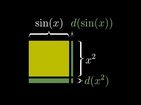
Visualizing the chain rule and product rule — 3Blue1Brown

Watch on YouTube

Open video on YouTube

Video

Implicit differentiation, what's going on here? — 3Blue1Brown

Watch on YouTube

Open video on YouTube

Video

Higher order derivatives — 3Blue1Brown

Watch on YouTube

Open video on YouTube

Two short Khan Academy clips build the specific picture of a partial derivative as the slope of a slice through a surface:

Video

Partial derivatives, introduction — Khan Academy

Watch on YouTube

Open video on YouTube

Video

Partial derivatives and graphs — Khan Academy

Watch on YouTube

Open video on YouTube

Websites

OpenStax, Calculus Volume 3, Chapter 4. 4.1 Functions of Several Variables, 4.3 Partial Derivatives and 4.5 The Chain Rule — many more worked examples than we have room for, with exercises.
Paul's Online Math Notes. Partial Derivatives and Chain Rule — the quickest source of extra practice once you know which technique you need. The chain-rule page is particularly good on tree diagrams for keeping track of which variable depends on which.

Remark

One thing you will not find in the calculus sources: the notation $\left(\frac{\partial T}{\partial p}\right)_V$ with an explicit subscript. Mathematics courses usually fix the independent variables once and never revisit the choice, so the ambiguity never arises. In thermodynamics it arises constantly, which is why this chapter labours the point. For that side of the subject a thermodynamics text will serve you better than a calculus one.