Chapter 1
Infinite Series and Power Series
1.1Definitions and Notation
A sequence is an ordered list of numbers:
Here is the first term and is the general term: the formula that tells us how to write down the th entry for any .
Examples of Sequences
The partial sum is the sum of the first terms of a sequence:
Each is an ordinary finite sum, so the partial sums themselves form a new sequence
Examples of Partial Sums
An infinite series is the sum of all terms in a sequence:
We cannot literally add infinitely many numbers, so this symbol is defined as the limit of the partial sums:
If that limit exists and is finite, the series converges to it; otherwise the series diverges. Every convergence test in this chapter is ultimately a statement about the sequence
Examples of Infinite Series
(read "n factorial") is defined as:
Example:
1.2Geometric Sequences and Series
A geometric sequence is a sequence in which each term is obtained by multiplying the previous one by a fixed number , called the common ratio:
Geometric series are conventionally indexed from , so that the general term is and the term itself corresponds to . Elsewhere in this chapter sequences start at . Always check which convention a formula assumes: the first terms of a geometric series run from up to , not up to .
Examples
Exponential Growth (e.g., Bacteria): with
Decay (e.g., Bouncing Ball): with
1.2.1Finite Geometric Series
The sum of the first terms of a geometric series is:
Consider the geometric series
Multiply both sides by :
Subtracting these two equations gives
Factor the left-hand side:
Finally, dividing both sides by (valid when ), we obtain
1.2.2Infinite Geometric Series
We do not need a new argument here: the infinite case follows from the finite formula we just proved by letting .
The series converges if and only if , and in that case
By definition (1.4) the sum is , and by the previous theorem
The only -dependent piece is . If then , so
If then and the limit does not exist; if then ; and if the partial sums oscillate between and . In each of these cases the series diverges.
So for the series diverges — it does not approach any finite value. Note that divergence does not always mean “blows up”: for the partial sums stay bounded but never settle down, and that is enough to diverge.
A ball is dropped from a height of yard and rebounds to of its previous height on each bounce. Find the total distance it travels.
Solution.
The initial drop covers yard and is counted once. After that, the ball rises to height and falls back through the same height, then rises to and falls back, and so on. Every bounce height is therefore traversed twice, which is where the factor of comes from:
The sum is geometric with first term and ratio . Since it converges, and by (1.12)
Therefore
Note that the ball bounces infinitely many times yet travels only a finite distance — infinitely many terms can still add up to a finite total.
This is a geometric series with :
The repeating part is geometric with:
Thus:
A beam of light of intensity strikes a glass plate. At each surface a fraction of the intensity is reflected and a fraction is transmitted. Find the total intensity that emerges from the far side, accounting for light that bounces back and forth inside the plate.
Solution.
Follow the beam through the plate:
It crosses the front surface, keeping a fraction , then crosses the back surface, keeping another . Emerging intensity: .
Alternatively it reflects off the back surface (), reflects off the front surface (), and then exits. Each such round trip costs a factor .
So the emerging beams have intensities
which is geometric with first term and ratio . Because we have , so by (1.12)
As a check: if (no reflection) then , as it must be. Note that the naive answer is too small — the multiple reflections matter.
1.3Limit of the General Term as
The limit of the general term of a sequence as is denoted by:
Evaluate:
Solution.
The highest power of is in both the numerator and the denominator (note that ), so divide both by . Inside the square root this means dividing by :
Now every term of the form tends to as , leaving
Evaluate:
Solution: Using L'Hôpital's Rule
Note: Although is discrete, the limit is evaluated using a continuous extension .
Evaluate:
Solution.
Take logarithm:
Hence:
1.4Testing Series for Convergence
1.4.1Preliminary Test
If , the series diverges.
If , further testing is required — the test says nothing either way.
Test the series
Solution.
The general term is . Dividing numerator and denominator by gives as . Since this limit is , the series diverges by the Preliminary Test.
1.4.2Comparison Test
Let be an unknown series with non-negative terms.
If there exists a convergent series such that
then converges.
If there exists a divergent series such that
then diverges.
Test for convergence.
Solution.
We compare against a geometric series. Both and are products of factors, but from the fourth factor onward every factor of is at least as large as the corresponding factor . Concretely, for ,
as one checks at () and which only improves as grows. Taking reciprocals reverses the inequality:
The geometric series has , so and it converges. Since the Comparison Test only requires the inequality to hold for all sufficiently large , it applies here and converges.
1.4.3Integral Test
Let where is positive, continuous, and decreasing for .
Then the infinite series
converges if and only if the improper integral
is finite.
Test the harmonic series .
Solution.
Let . On this function is positive, continuous, and decreasing, so the Integral Test applies. Evaluating the improper integral as a limit:
The integral is infinite, so by the Integral Test the harmonic series diverges.
This result is worth remembering. The terms tend to , yet the series still diverges — proof that alone is never enough to conclude convergence.
For a constant ,
For the terms do not tend to , so the series diverges by the Preliminary Test. For the function is positive, continuous, and decreasing on , so the Integral Test applies. The case is the harmonic series just treated. For ,
If the exponent is negative, so and the integral equals , which is finite: the series converges. If the exponent is positive, , and the series diverges.
The -series and the geometric series are the two standard yardsticks against which unknown series are measured in the Comparison and Limit Comparison Tests. In particular converges () while diverges ().
1.4.4Ratio Test
Let
Then
Test , a sum of the kind that arises when computing average energies from a partition function.
Solution.
Here . Form the ratio, remembering that dividing by means multiplying by its reciprocal:
Since , we get
so the series converges by the Ratio Test. Notice the general lesson: an exponential in the denominator beats any power of in the numerator.
The Ratio Test is the natural first choice whenever contains factorials or th powers, because those are exactly the expressions that simplify when is divided by . It is of no use for -series: for one finds , and the test is inconclusive.
1.4.5Limit Comparison Test
If
then the two series and either both converge or both diverge.
Test
for convergence.
Solution.
Keep only the highest power of in each part. In the numerator , and in the denominator . So for large
This suggests comparing with . Forming the required limit,
which satisfies . Since is a -series with it converges, so the given series converges by the Limit Comparison Test.
1.5Alternating Series
Many series we have studied so far have non-negative terms. We now consider an important class of series whose terms alternate in sign.
A series is called alternating if the signs of its terms switch between positive and negative, for example
Equivalently, it may be written in the form
An alternating series of the form (1.53)
converges if
1.5.1Absolute vs. Conditional Convergence
If converges, the series is said to converge absolutely.
If converges but diverges, then is conditionally convergent.
If converges, then converges.
This theorem is what makes the definition useful. All of the tests in Section 1.4 require non-negative terms, so they cannot be applied directly to a series with mixed signs. The theorem provides the way around this: apply the tests to instead, and if that converges, the original series converges too. In practice the Ratio Test is used this way constantly — note that it was already stated in terms of for exactly this reason.
Test for convergence.
Solution.
The terms alternate in sign, so no comparison or integral test applies directly. Take absolute values:
which is a -series with and therefore converges by (1.42). Since converges, the theorem above tells us the original series converges — and it converges absolutely.
Consider from (1.54).
Solution.
Set . Then for all , and , so both conditions in (1.56) hold and the series converges by the Alternating Series Test.
However, taking absolute values gives , the harmonic series, which diverges. The series therefore converges but not absolutely: it is conditionally convergent. Its sum is .
The distinction is not merely bookkeeping. The terms of an absolutely convergent series may be rearranged freely without changing the sum, exactly as with a finite sum. This is false for a conditionally convergent series: by reordering the alternating harmonic series one can make it converge to any number at all. Whenever you reorder, split, or term-by-term combine infinite series, absolute convergence is the property that makes it legitimate.
Summary: Convergence Tests
The tests of this section are collected below. A second table, covering every kind of series met in the chapter, appears at the end.
| Test | Key Idea | Best used when |
| Preliminary Test | If , the series diverges. | Always try this first. |
| Comparison Test | Compare to a known convergent or divergent series. | resembles a -series or geometric series. |
| Integral Test | Integrate corresponding to . | is easy to integrate. |
| Ratio Test | Use . | contains factorials or th powers. |
| Limit Comparison Test | Compare using . | is a ratio of polynomials or roots. |
| Alternating Series Test | decreasing and . | Terms alternate in sign. |
| Absolute Convergence | Apply the tests above to . | Terms have mixed signs. |
Nearly every comparison comes back to one of these:
1.7Power Series
A power series centered at is an infinite series of the form
where:
are constants called the coefficients,
is the center of the series,
is the variable.
When the center is the series takes the simpler form , called a power series in .
A power series is not a single number but a function of : for each value of we get a different series of constants, which may converge or diverge. The first question about any power series is therefore for which does it converge? That is what the next subsection answers.
1.7.1Radius and Interval of Convergence
For a power series , there exists a real number , called the radius of convergence, such that:
The series converges absolutely when ;
The series diverges when ;
When , convergence must be checked separately.
If
with conventions: and .
Find the radius and interval of convergence of
Solution.
The series is centred at with . Apply the ratio formula for :
so and . The series therefore converges for , that is .
The endpoints must be checked one at a time, by substituting them into the original series:
At : , giving . This alternates, its terms decrease, and , so it converges by the Alternating Series Test. It does not converge absolutely (see the next endpoint), so convergence here is conditional.
At : , giving . This behaves like a -series with , so it diverges.
One endpoint is included and the other is not:
Find the radius and interval of convergence of
Solution.
Here , so
so and . Convergence therefore holds for , that is .
At the endpoints, substitute into the original series and let the cancel:
At : , so the term is . This is the alternating harmonic series, which converges — but only conditionally, since taking absolute values gives the divergent harmonic series.
At : , so the term is . This is the harmonic series, which diverges.
Hence the interval of convergence is
Notice what happened at the endpoints above. It is tempting to look only at , see the in the denominator, and conclude that both endpoints converge absolutely. That is wrong: at an endpoint the factor contributes , which cancels the and leaves the harmonic series behind. Always substitute the endpoint into the full term , never into alone.
At the endpoints, you often use the Alternating Series Test or comparison with a -series to decide convergence.
1.8Theorems About Power Series
Suppose
has radius of convergence . Then for every with , the following properties hold:
Differentiation and Integration. The series for may be differentiated or integrated term by term:
(1.68)Both resulting power series have the same radius of convergence .
Algebra of Series. Power series may be added, subtracted, and multiplied term by term. The resulting series converges at least in the intersection of the original intervals of convergence. Division is valid provided the denominator does not vanish at the center ; if a factor cancels (e.g. ), a power-series representation still exists.
Substitution. If is a function such that , then
(1.69)Uniqueness. A power series represents a unique function on its interval of convergence, and the coefficients satisfy
(1.70)
1.9Taylor and Maclaurin Series
Finding the Coefficients
Suppose a function can be expressed as a power series about :
Differentiating term by term yields
Evaluating successively at gives
Therefore, in general,
If has derivatives of all orders in an open interval containing , then
for every in the interval where the series converges. This is called the Taylor series of about .
Assume can be written as a power series about . Term-by-term differentiation, as carried out above, forces
Substituting these coefficients into the original power series yields
Read the proof carefully: it assumes that equals some power series, and then shows the coefficients could only be . So it establishes uniqueness, not existence. It does not show that the Taylor series of an arbitrary actually converges back to .
That distinction is real. The function
has derivatives of every order at , and every one of them is zero. Its Maclaurin series is therefore , which converges everywhere but equals only at the single point .
A function that does equal its Taylor series on an interval is called analytic. Every function we expand in this chapter — , , , , — is analytic on the interval stated, so in practice you may expand freely. Just do not mistake “infinitely differentiable” for “equal to its Taylor series”.
A Maclaurin series is a Taylor series centered at :
Find the Maclaurin series for .
Solution.
Differentiate repeatedly. The derivatives of repeat with period four, so we only ever need these four:
and then the pattern repeats. Substituting into , every even power drops out because its coefficient is zero:
Only odd powers survive, with alternating signs, so
The Ratio Test confirms : the factorial in the denominator grows faster than any power of , so the series converges for every .
That contains only odd powers is no accident. makes it an odd function, and only odd powers of are odd functions. Likewise is even and its series below contains only even powers. This is a quick way to catch algebra errors: if an even power appears in a series for an odd function, something has gone wrong.
A pendulum of length swinging through an angle from the vertical obeys
where is the acceleration due to gravity. This equation cannot be solved in terms of elementary functions. Show how a series expansion rescues the situation for small swings.
Solution.
The obstacle is the on the right, which makes (1.83) nonlinear. Replace it by its Maclaurin series:
For a small swing, is small and each successive term is far smaller than the one before. Keeping only the first term gives the small-angle approximation , and (1.83) becomes
which is linear and has the familiar oscillating solution with . This is simple harmonic motion, and it is where the standard pendulum period comes from.
How good is the approximation? The first term we discarded is , so the relative error is about . For a swing of radians that is roughly . Note that must be in radians — the series is only valid in radians, which is the real reason radians are the natural unit for angles in physics.
Common Maclaurin Series
Memorise these five. Almost every series in this chapter, and most you will meet later, is obtained from one of them by substitution, differentiation, integration, or multiplication — the techniques of the next section — rather than by computing derivatives from scratch.
Note the endpoint in : the series does converge at , where it gives the alternating harmonic series and hence , as promised in Section 1.4. It diverges at , where it becomes the harmonic series. The interval is genuinely lopsided, which is why it is written rather than .
1.10Techniques for Obtaining Power Series Expansions
Power series expansions can be generated or modified using several systematic techniques. These allow you to construct new series from known ones without starting from scratch.
1.10.1Using Differentiation and Integration
Start with the geometric series for :
Differentiate term-by-term:
Integrate term-by-term:
Both series have radius .
At , the differentiated or integrated series may behave differently from the original. Endpoint behavior must be checked separately.
1.10.2Multiplying a Series by a Polynomial or by Another Series
If
and is a polynomial, then is obtained by multiplying through the series term-by-term and combining like powers. Similarly, two infinite series can be multiplied by forming their Cauchy product and collecting like powers of .
To find the series for , we multiply the Maclaurin series for by :
Expanding and combining like terms:
Thus, the series begins
This illustrates how multiplying a series by a polynomial simply shifts and rescales its terms. Notice that this method is easier than computing successive derivatives of to form its Taylor series directly.
To find the series for , multiply the Maclaurin series for and :
Work power by power. For each power of , collect every way of forming it as (term from ) (term from ):
Thus the series begins
Note that the term cancels exactly. Two warnings: include every product contributing to a given power (the row has three), and do not carry higher-order terms you will only discard — to reach you never need a term beyond from either factor.
1.10.3Division of Two Series or of a Series by a Polynomial
If and , you can perform long division or solve for coefficients by matching powers. The second method is usually less error-prone: write the unknown quotient with undetermined coefficients, multiply back up, and match powers of one at a time.
Find the Maclaurin series for up to .
Solution.
Rather than differentiate five times, divide the known series
Since is odd and , only odd powers can appear. Write
and clear the denominator using :
Now match coefficients power by power:
Therefore
Unlike and , this series does not converge for all : vanishes at , where blows up, so . Dividing by a series always risks a smaller radius of convergence than either series started with.
1.10.4Using the Binomial Series
For any real or complex exponent ,
where the generalized binomial coefficients are given by
The series converges for , and may converge at depending on the value of .
The letter here is the binomial exponent and has nothing to do with the of the -series in Section 1.4. The clash is unfortunate but standard; the meaning is always clear from context.
Find the series for .
Solution.
Here , so the coefficients are
Substituting into the binomial series — note that the signs are already carried by the coefficients, so we do not insert extra alternating signs by hand:
This is a useful check on the whole binomial machinery: the answer is just the geometric series with ratio , which we already knew from Section 1.4.
Expand .
Solution.
Here , so . Compute the first few coefficients directly from the definition, each being a product of factors divided by :
Hence
Only the first two terms are needed in most applications: for small , .
The exact potential energy of a mass at height above the surface of the Earth (radius , mass ) is
where is the gravitational constant. The familiar classroom formula is . Reconcile the two.
Solution.
The exact expression depends on in an awkward way. Factor out so that the -dependence sits in a small quantity:
Near the Earth's surface — even a tall mountain has — so is small and the binomial series with applies:
Therefore
The first term does not depend on ; since only changes in potential energy are physically meaningful, it can be discarded by choosing where to put the zero of energy. The second term is exactly , and it identifies — the surface gravity is not an independent constant of nature but the first series coefficient of the true potential.
The next term is smaller by a factor , so for km the error in using is about . This is the same pattern as the relativistic kinetic energy of Section 1.11: the simple formula is the first term of a series, accurate whenever the neglected ratio is small.
For nonnegative integers , the binomial expansion terminates after , giving the usual finite binomial theorem. For non-integers , the series is infinite and converges for .
1.10.5Substitution of a Polynomial or a Series into Another Series
From , substitute :
Find the Maclaurin series of up to .
First, use
Let . Then
Compute powers of to the needed order:
Substitute:
(The radius of convergence is limited by the nearest pole of , so .)
Any manipulation such as multiplication, differentiation, integration, or substitution can alter the radius of convergence. Always verify the new convergence interval after such operations.
1.10.6Combination of Methods
You can combine multiplication, division, substitution, differentiation, and integration.
Find the Maclaurin series for .
We use the identity
First, expand the denominator as a binomial series:
Now integrate term by term:
Thus,
The expansion of is valid only for , so integration gives ; the endpoints survive because there the series becomes alternating with terms decreasing to zero. Setting gives the celebrated
a beautiful formula but a hopeless way to compute : it converges so slowly that several hundred terms are needed for two decimal places.
1.10.7Taylor Series Using Basic Maclaurin Series
Taylor’s theorem:
gives the coefficients directly from derivatives at .
Expand about :
Let , so :
Thus:
1.11Applications of Series
In the example of the bouncing ball, we saw that the sum of an infinite series can often be very close to the sum of a finite number of initial terms. This principle underlies many applications:
Many real-world problems cannot be solved exactly but can be expressed as an infinite series.
In practice, only as many terms as needed to achieve the desired accuracy are computed.
Series solutions are commonly used in solving:
ordinary differential equations (Chapters 8 and 12),
partial differential equations (Chapter 13).
Approximating Functions
If a function is analytic, cutting its Taylor series off after a few terms gives a polynomial approximation whose accuracy improves with each term kept.
Approximate using the binomial series.
Solution.
Write with , and use the expansion found above (the binomial series with ):
Substituting term by term:
The true value is , so three terms already give an error of about . Observe how fast the terms shrink: each is roughly times the one before. This is typical — when the expansion variable is small, a couple of terms suffice.
Recovering Simple Physical Laws
The examples below show the pattern that recurs throughout physics: an exact formula is awkward, but its first few series terms are both simple and accurate in the regime of interest. We have already seen two instances — the small-angle pendulum in Section 1.9 and gravitational potential energy in Section 1.10.
The exact relativistic kinetic energy of a particle of mass moving at speed is
Show that at everyday speeds this reduces to the familiar .
Solution.
Write , so that . For small ,
Substituting and cancelling the :
The leading term is exactly the Newtonian kinetic energy. The first correction is smaller than it by a factor , which for a jet aircraft ( m/s) is about — utterly negligible. Newtonian mechanics is not a different theory here; it is the first term of a series.
A hot object emits light across a range of frequencies. Planck's law gives the energy radiated at frequency by a body at absolute temperature as
where is Planck's constant and is Boltzmann's constant. Before Planck, the accepted classical result was the Rayleigh–Jeans law . Show that Planck's law reduces to it at low frequencies.
Solution.
The physically meaningful comparison is between the photon energy and the thermal energy . “Low frequency” means , so set
and expand the exponential in the denominator using the Maclaurin series for :
Note that the leading cancels exactly; this is why the expansion is needed rather than simply setting , which would give a useless in the denominator. Substituting into (1.135):
which is exactly the Rayleigh–Jeans law. So the classical result was never wrong, only incomplete: it is the leading term of Planck's law when . At high frequencies the neglected terms dominate, the exponential suppresses , and Planck's law avoids the “ultraviolet catastrophe” — the classical prediction that a hot body radiates infinite total energy.
Series such as (1.133), written in powers of , are the power series of Section 1.7. Beyond the approximations above, they are used to define:
Functions of complex numbers (Chapter 2, Section 8),
Functions of matrices (Chapter 3, Section 6),
Fourier series (Chapter 7),
Special functions like Legendre and Bessel functions (Chapters 12 and 13).
Summary: Types of Series
The table below collects every kind of series met in this chapter, together with Fourier series, which are taken up in Chapter 7.
| Category | Example Formula | Main Feature / Description |
| Arithmetic | Constant difference between terms. | |
| Geometric | Constant ratio ; converges iff . | |
| Harmonic | Reciprocals of the positive integers; the case of a -series. Diverges. | |
| -Series | Converges for , diverges for . | |
| Alternating | Signs alternate; may converge conditionally. | |
| Power Series | Converges on an interval around . | |
| Taylor Series | Power-series representation of an analytic function. | |
| Maclaurin Series | Taylor series centred at . | |
| Binomial Series | Valid for any real or complex , with . | |
| Fourier Series | Represents periodic functions using sines and cosines. |
For the Interested Reader
Everything in this chapter is standard first-year material, so if a topic did not settle the first time, a second presentation of it often helps. Everything listed below is free to read or watch. The material is grouped the way the chapter is: first convergence, then power series.
Convergence of series
Sections 1.4 and the alternating-series material that follows it.
OpenStax, Calculus Volume 2, Chapter 5. A full textbook treatment in almost our order — 5.1 Sequences, 5.2 Infinite Series, 5.3 Divergence and Integral Tests, 5.4 Comparison Tests, 5.5 Alternating Series, 5.6 Ratio and Root Tests — the last of which also covers the Root Test, which we did not.
Paul's Online Math Notes. The fastest place to see a test applied several times in a row: Series \& Sequences and, especially, Strategy for Series — a decision procedure for choosing a test, and a good companion to our summary table.
Khan Academy. Series (AP Calculus BC) — short videos, each followed by practice questions. Best for drilling the convergence tests until they are automatic.
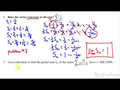
On what it actually means for an infinite sum to have a value:
Defining Convergent and Divergent Infinite Series
 Watch on YouTube
Power series, Taylor and Maclaurin
OpenStax, Calculus Volume 2, Chapter 6. 6.1 Power Series and Functions and 6.2 Properties of Power Series cover Sections 1.7 and 1.8; 6.3 Taylor and Maclaurin Series covers Section 1.9 and, unlike us, treats the remainder term properly; 6.4 Working with Taylor Series has the binomial series and further approximations.
Paul's Online Math Notes. Power Series — many more interval-of-convergence problems, including the endpoint checks that catch people out — and Taylor Series.
A visual account of why the coefficients involve derivatives and factorials. Worth twenty minutes if felt like something you memorised rather than understood:
Taylor Series — 3Blue1Brown, Essence of Calculus, Chapter 11
 Watch on YouTube
One caution when reading elsewhere. These are calculus sources, so they emphasise proving whether a series converges. In this course convergence is usually the easy part: what we actually want is the value of the sum, or a few terms of it accurate enough to use, as in the relativistic kinetic energy example of Section 1.11. Read them for the machinery, but keep our purpose in mind.