Chapter 6

Vector Analysis

6.1Applications of Vector Multiplication

Dot Product (Scalar Product)

Definition - Dot Product

For two vectors \(\vec{A}\) and \(\vec{B}\),

\begin{equation} \boxed{\vec{A}\cdot\vec{B}=A_xB_x+A_yB_y+A_zB_z = AB\cos\theta,} \end{equation}

where \(\theta\) is the angle between \(\vec{A}\) and \(\vec{B}\).

Remark

The dot product measures how much of one vector lies along another. It is maximal when the vectors are parallel and zero when they are perpendicular.

Theorem - Properties of the Dot Product
  1. Commutative: \(\vec{A}\cdot\vec{B}=\vec{B}\cdot\vec{A}\).

  2. Distributive: \(\vec{A}\cdot(\vec{B}+\vec{C})=\vec{A}\cdot\vec{B}+\vec{A}\cdot\vec{C}\).

  3. Scalar multiplication: \((m\vec{A})\cdot\vec{B}=m(\vec{A}\cdot\vec{B})\).

  4. \(\vec{A}\cdot\vec{A}=|\vec{A}|^2\).

Example - Work done by a constant force

If a force \(\vec{F}\) moves a particle through a displacement \(\vec{r}\), the work done is

\begin{equation} W=\vec{F}\cdot\vec{r}=Fr\cos\theta. \end{equation}

Only the component of \(\vec{F}\) in the direction of motion contributes to the work.
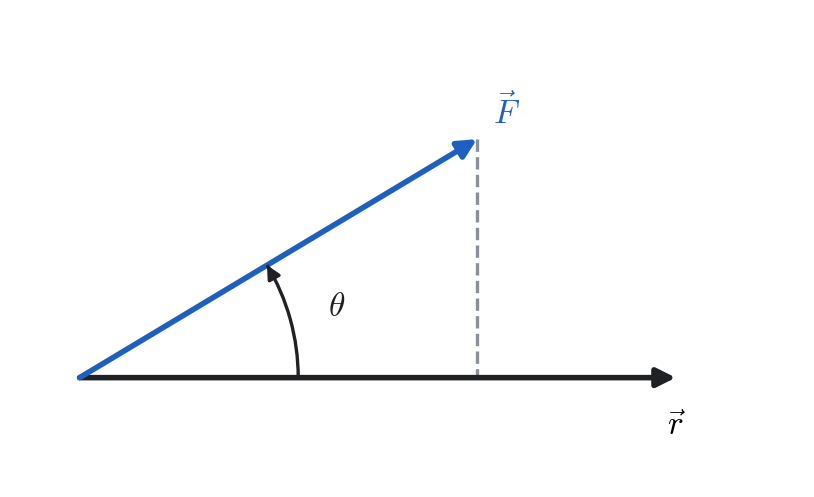
Work as a dot product: only the component of F along the displacement contributes.
Figure 6.1. Work as a dot product: only the component of \(\vec{F}\) along the displacement contributes.

Cross Product (Vector Product)

Definition - Cross Product

For two vectors \(\vec{A}\) and \(\vec{B}\),

\begin{equation} \boxed{ \vec{A}\times\vec{B}= \begin{vmatrix} \hat{i}&\hat{j}&\hat{k}\\ A_x&A_y&A_z\\ B_x&B_y&B_z \end{vmatrix} = (A_yB_z-A_zB_y)\hat{i}+(A_zB_x-A_xB_z)\hat{j}+(A_xB_y-A_yB_x)\hat{k}. } \end{equation}

The magnitude is \(|\vec{A}\times\vec{B}|=AB\sin\theta\), and the direction is given by the right-hand rule.

Remark

The vector \(\vec{A}\times\vec{B}\) is perpendicular to both \(\vec{A}\) and \(\vec{B}\). If the two vectors are parallel or antiparallel, their cross product is zero.

Theorem - Properties of the Cross Product
  1. Anti-commutative: \(\vec{A}\times\vec{B}=-\vec{B}\times\vec{A}\).

  2. Distributive: \(\vec{A}\times(\vec{B}+\vec{C})=\vec{A}\times\vec{B}+\vec{A}\times\vec{C}\).

  3. \((m\vec{A})\times\vec{B}=m(\vec{A}\times\vec{B})\).

  4. \(\vec{A}\times\vec{A}=0\).

Example - Torque

A force \(\vec{F}\) applied at position vector \(\vec{r}\) produces a torque

\begin{equation} \vec{\tau}=\vec{r}\times\vec{F}. \end{equation}

Its magnitude \(|\vec{\tau}|=rF\sin\theta\) equals the product of the force and its perpendicular lever arm.

Scalar Triple Product

Definition - Scalar Triple Product
\begin{equation} \boxed{ \vec{A}\cdot(\vec{B}\times\vec{C})= \begin{vmatrix} A_x & A_y & A_z\\ B_x & B_y & B_z\\ C_x & C_y & C_z \end{vmatrix}. } \end{equation}

This scalar represents the signed volume of the parallelepiped formed by \(\vec{A}\), \(\vec{B}\), and \(\vec{C}\).

Remark

If \(\vec{A}\cdot(\vec{B}\times\vec{C})=0\), the three vectors are coplanar. The sign of this product distinguishes right-handed and left-handed orientations.

Theorem - Properties of the Scalar Triple Product
  1. Cyclic permutation: \(\vec{A}\cdot(\vec{B}\times\vec{C})=\vec{B}\cdot(\vec{C}\times\vec{A})=\vec{C}\cdot(\vec{A}\times\vec{B})\).

  2. Interchanging any two vectors reverses the sign.

  3. The absolute value equals the geometric volume of the parallelepiped.

Example - Volume of a parallelepiped

Let \(\vec{A}=(1,2,3)\), \(\vec{B}=(2,1,1)\), and \(\vec{C}=(1,1,0)\). Then

\begin{equation} V=\vec{A}\cdot(\vec{B}\times\vec{C}) =\begin{vmatrix} 1&2&3\\ 2&1&1\\ 1&1&0 \end{vmatrix} =4. \end{equation}

Hence, the volume of the parallelepiped is \(V=4\) (unit)\(^3\).

Vector Triple Product

Definition - Vector Triple Product
\begin{equation} \boxed{ \vec{A}\times(\vec{B}\times\vec{C}) =\vec{B}(\vec{A}\cdot\vec{C})-\vec{C}(\vec{A}\cdot\vec{B}). } \end{equation}

This identity is commonly known as the BAC–CAB rule. The resulting vector lies in the plane of \(\vec{B}\) and \(\vec{C}\).

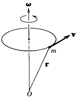
A particle of mass m in rigid rotation about an axis through O with angular velocity , at position r and moving with velocity v.
Figure 6.2. A particle of mass \(m\) in rigid rotation about an axis through \(O\) with angular velocity \(\vec{\omega}\), at position \(\vec{r}\) and moving with velocity \(\vec{v}\).
Example - Angular Momentum for Rigid Rotation

For a particle in rigid rotation with angular velocity \(\vec{\omega}\), the velocity is

\begin{equation} \vec{v} = \vec{\omega} \times \vec{r}. \end{equation}

The linear momentum is \(\vec{p} = m\vec{v} = m(\vec{\omega} \times \vec{r})\). Hence the angular momentum is

\begin{equation} \vec{L} = \vec{r} \times \vec{p} = m\,\vec{r} \times (\vec{\omega} \times \vec{r}). \end{equation}

Using the vector triple–product identity,

\begin{equation} \vec{r} \times (\vec{\omega} \times \vec{r}) = \vec{\omega}(\vec{r} \cdot \vec{r}) - \vec{r}(\vec{r} \cdot \vec{\omega}) = r^{2}\vec{\omega} - (\vec{r} \cdot \vec{\omega})\vec{r}. \end{equation}

Therefore,

\begin{equation} \boxed{\vec{L} = m\big[r^{2}\vec{\omega} - (\vec{r} \cdot \vec{\omega})\vec{r}\big]}. \end{equation}

If the rotation axis is perpendicular to \(\vec{r}\), then \(\vec{r} \cdot \vec{\omega}=0\) and

\begin{equation} \vec{L}=m r^{2}\vec{\omega}. \end{equation}

This form shows that the angular momentum is parallel to the angular velocity, with magnitude proportional to the moment of inertia \(I=m r^{2}\).

6.2Differentiation of Vectors

In physics, many vector quantities—such as position, velocity, and acceleration—vary with time or with spatial coordinates. We therefore need rules for differentiating and integrating vectors.

Definition - Derivative of a Vector

If a vector \(\vec{A}\) depends on a variable \(t\), its derivative with respect to \(t\) is defined as

\begin{equation} \frac{d \vec{A}}{d t} = \lim_{\Delta t \to 0} \frac{\vec{A}(t+\Delta t) - \vec{A}(t)}{\Delta t}. \end{equation}

The derivative \(\frac{d \vec{A}}{d t}\) is itself a vector, representing the rate of change of \(\vec{A}\).

If the components of \(\vec{A}\) are differentiable functions of \(t\),

\begin{equation} \vec{A}(t)=A_x(t)\hat{i}+A_y(t)\hat{j}+A_z(t)\hat{k}, \end{equation}

then

\begin{equation} \frac{d \vec{A}}{d t} = \frac{d A_x}{d t}\hat{i}+\frac{d A_y}{d t}\hat{j}+\frac{d A_z}{d t}\hat{k}. \end{equation}
Remark

The derivative of a vector may change the magnitude, the direction, or both. For instance, in uniform circular motion, \(|\vec{r}|\) is constant but \(\vec{r}\) changes direction continuously, producing a nonzero \(\frac{d \vec{r}}{d t}\).

Example - Velocity and Acceleration in Different Coordinate Systems

1) Cartesian Coordinates \((x, y, z)\).

Position vector:

\begin{equation} \vec{r} = x\,\hat{i} + y\,\hat{j} + z\,\hat{k}. \end{equation}

Differential displacement:

\begin{equation} d\vec{r} = \hat{i}\,dx + \hat{j}\,dy + \hat{k}\,dz. \end{equation}

Velocity (divide by \(dt\)):

\begin{equation} \boxed{ \vec{v} = \frac{d \vec r}{d t} = \frac{dx}{dt}\,\hat{i} + \frac{dy}{dt}\,\hat{j} + \frac{dz}{dt}\,\hat{k}. } \end{equation}

Interpretation:

\begin{equation} \begin{aligned} v_x &= \frac{dx}{dt} \quad &\text{linear velocity in the $x$-direction},\\[4pt] v_y &= \frac{dy}{dt} \quad &\text{linear velocity in the $y$-direction},\\[4pt] v_z &= \frac{dz}{dt} \quad &\text{linear velocity in the $z$-direction}. \end{aligned} \end{equation}

2) Cylindrical Coordinates \((\rho, \phi, z)\).

Position vector:

\begin{equation} \vec{r} = \rho\,\hat{\rho} + z\,\hat{z}. \end{equation}

Differential displacement:

\begin{equation} \boxed{d\vec{r} = \hat{\rho}\,d\rho + \rho\,\hat{\phi}\,d\phi + \hat{z}\,dz.} \end{equation}

Velocity (divide by \(dt\)):

\begin{equation} \boxed{ \vec{v} = \frac{d \vec r}{d t} = \frac{d\rho}{dt}\,\hat{\rho} + \rho\,\frac{d\phi}{dt}\,\hat{\phi} + \frac{dz}{dt}\,\hat{z}. } \end{equation}

Interpretation:

\begin{equation} \begin{aligned} v_{\rho} &= \frac{d\rho}{dt} &\text{linear velocity in the radial direction},\\[4pt] v_{\phi} &= \rho\,\frac{d\phi}{dt} &\text{tangential (angular) velocity around the $z$-axis},\\[4pt] v_{z} &= \frac{dz}{dt} &\text{linear velocity along the $z$-axis}. \end{aligned} \end{equation}

3) Spherical Coordinates \((r, \theta, \phi)\).

Position vector:

\begin{equation} \vec{r} = r\,\hat{r}. \end{equation}

Differential displacement:

\begin{equation} \boxed{d\vec{r} = \hat{r}\,dr + r\,\hat{\theta}\,d\theta + r\sin\theta\,\hat{\phi}\,d\phi.} \end{equation}

Velocity (divide by \(dt\)):

\begin{equation} \boxed{ \vec{v} = \frac{d \vec r}{d t} = \frac{dr}{dt}\,\hat{r} + r\,\frac{d\theta}{dt}\,\hat{\theta} + r\sin\theta\,\frac{d\phi}{dt}\,\hat{\phi}. } \end{equation}

Interpretation:

\begin{equation} \begin{aligned} v_{r} &= \frac{dr}{dt} &\text{radial velocity (rate of change of distance from origin)},\\[4pt] v_{\theta} &= r\,\frac{d\theta}{dt} &\text{polar velocity (change in inclination)},\\[4pt] v_{\phi} &= r\sin\theta\,\frac{d\phi}{dt} &\text{azimuthal velocity (rotation around the $z$-axis)}. \end{aligned} \end{equation}
Theorem - Rules of Vector Differentiation
  1. \begin{equation} \frac{d}{dt}(\vec{A}+\vec{B}) = \frac{d\vec{A}}{dt} + \frac{d\vec{B}}{dt}. \end{equation}
  2. \begin{equation} \frac{d}{dt}(m\vec{A}) = \frac{dm}{dt}\,\vec{A} + m\frac{d\vec{A}}{dt}, \qquad \text{where $m$ is a scalar function of $t$.} \end{equation}
  3. \begin{equation} \frac{d}{dt}(\vec{A}\cdot\vec{B}) = \frac{d\vec{A}}{dt}\cdot\vec{B} + \vec{A}\cdot\frac{d\vec{B}}{dt}. \end{equation}
  4. \begin{equation} \frac{d}{dt}(\vec{A}\times\vec{B}) = \frac{d\vec{A}}{dt}\times\vec{B} + \vec{A}\times\frac{d\vec{B}}{dt}. \end{equation}
Example - Time derivative of angular momentum

The angular momentum of a particle is \(\vec{L} = \vec{r}\times m\vec{v}\). Then,

\begin{equation} \frac{d \vec{L}}{d t} = \frac{d \vec{r}}{d t}\times m\vec{v} + \vec{r}\times m\frac{d \vec{v}}{d t} = \vec{r}\times m\vec{a}. \end{equation}

The quantity \(\frac{d \vec{L}}{d t}\) is the torque \(\vec{\tau}\):

\begin{equation} \boxed{\vec{\tau}=\frac{d \vec{L}}{d t}}. \end{equation}

6.3Fields

Many physical quantities depend on position in space. Temperature, pressure, electric field, and magnetic field are examples of fields.

Definition - Scalar Field and Vector Field
  • A scalar field assigns a scalar value to every point in space:

    \begin{equation} \phi = \phi(x,y,z). \end{equation}

    Examples: temperature, electric potential, mass density.

  • A vector field assigns a vector to every point in space:

    \begin{equation} \vec{A}=\vec{A}(x,y,z)=A_x(x,y,z)\hat{i}+A_y(x,y,z)\hat{j}+A_z(x,y,z)\hat{k}. \end{equation}

    Examples: velocity field of a fluid, electric and magnetic fields.

Remark

At each point \((x,y,z)\), the scalar field gives one number, while the vector field gives three component functions that can vary continuously throughout space.

Example - Electric Field

For a point charge \(q\) at the origin,

\begin{equation} \vec{E}(\vec{r}) = \frac{1}{4\pi\varepsilon_0}\frac{q}{r^2}\hat{r}. \end{equation}

The direction of \(\vec{E}\) is radial, outward for \(q>0\) and inward for \(q<0\).

6.4Directional Derivative and Gradient

When a scalar field \(\phi(x,y,z)\) varies in space, we often wish to know the rate at which it changes in a given direction.

Definition - Directional Derivative

If \(\hat{u}\) is a unit vector specifying a direction, the rate of change of \(\phi\) in that direction is

\begin{equation} \boxed{ \frac{d \phi}{d s} = \vec{\nabla}\phi\cdot\hat{u} = \frac{\partial \phi}{\partial x}u_x + \frac{\partial \phi}{\partial y}u_y + \frac{\partial \phi}{\partial z}u_z, } \end{equation}

where \(s\) measures distance along \(\hat{u}\).

Definition - Gradient of a Scalar Field

The gradient of \(\phi\) is the vector field

\begin{equation} \boxed{ \vec{\nabla}\phi = \frac{\partial \phi}{\partial x}\hat{i} + \frac{\partial \phi}{\partial y}\hat{j} + \frac{\partial \phi}{\partial z}\hat{k}. } \end{equation}
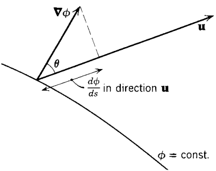
The gradient is perpendicular to the level curve =const, and its projection on a direction u is the directional derivative d/ds in that direction.
Figure 6.3. The gradient \(\vec{\nabla}\phi\) is perpendicular to the level curve \(\phi=\text{const}\), and its projection on a direction \(\vec{u}\) is the directional derivative \(d\phi/ds\) in that direction.
Remark

The gradient \(\vec{\nabla}\phi\) points in the direction of maximum increase of \(\phi\), and its magnitude \(|\vec{\nabla}\phi|\) gives the maximum rate of increase per unit distance.

Example - Directional Derivative

Find the directional derivative of

\begin{equation} \phi = x^2y + xz \end{equation}

at the point \((1,2,-1)\) in the direction of the vector

\begin{equation} \vec{A} = 2\hat{i} - 2\hat{j} + \hat{k}. \end{equation}

Step 1: Determine the unit vector in the direction of \(\vec{A}\).

\begin{equation} |\vec{A}| = \sqrt{2^2 + (-2)^2 + 1^2} = 3, \qquad \hat{u} = \frac{\vec{A}}{|\vec{A}|} = \frac{1}{3}(2\hat{i} - 2\hat{j} + \hat{k}). \end{equation}

Step 2: Compute the gradient of \(\phi\).

\begin{equation} \vec{\nabla} \phi = \hat{i}\,\frac{\partial \phi}{\partial x} + \hat{j}\,\frac{\partial \phi}{\partial y} + \hat{k}\,\frac{\partial \phi}{\partial z}. \end{equation}

Since \(\phi = x^2y + xz\),

\begin{equation} \frac{\partial \phi}{\partial x} = 2xy + z, \qquad \frac{\partial \phi}{\partial y} = x^2, \qquad \frac{\partial \phi}{\partial z} = x. \end{equation}

Hence

\begin{equation} \boxed{\vec{\nabla}\phi = (2xy + z)\,\hat{i} + x^2\,\hat{j} + x\,\hat{k}.} \end{equation}

At the point \((1,2,-1)\):

\begin{equation} \vec{\nabla}\phi(1,2,-1) = (2(1)(2) - 1)\,\hat{i} + (1)^2\,\hat{j} + (1)\,\hat{k} = 3\hat{i} + \hat{j} + \hat{k}. \end{equation}

Step 3: Compute the directional derivative.

The directional derivative of \(\phi\) in the direction \(\hat{u}\) is given by

\begin{equation} \boxed{ \frac{d \phi}{d s} = \vec{\nabla}\phi \cdot \hat{u}. } \end{equation}

Substitute:

\begin{equation} \frac{d \phi}{d s} = (3\hat{i} + \hat{j} + \hat{k}) \cdot \frac{1}{3}(2\hat{i} - 2\hat{j} + \hat{k}) = \frac{1}{3}(6 - 2 + 1) = \frac{5}{3}. \end{equation}

Answer:

\begin{equation} \boxed{\left(\frac{d \phi}{d s}\right)_{(1,2,-1)} = \frac{5}{3}.} \end{equation}

Gradient as a Normal to a Surface

Remark

If we consider a surface \(\phi(x,y,z)=\text{constant}\), and let \(\hat{t}\) be a unit tangent vector to this surface at some point, then the directional derivative of \(\phi\) along the tangent direction is zero:

\begin{equation} \frac{d \phi}{d s} = \vec{\nabla}\phi \cdot \hat{t} = 0. \end{equation}

Hence, \(\vec{\nabla}\phi\) is perpendicular to all tangent directions and therefore

\begin{equation} \boxed{\vec{\nabla}\phi \ \text{is a vector normal to the surface} \ \phi(x,y,z)=\text{constant}.} \end{equation}
Example - Tangent Plane and Normal Line to a Sphere

Find the equations of the tangent plane and the normal line to the surface of a sphere

\begin{equation} \phi(x,y,z) = x^2 + y^2 + z^2 = a^2 \end{equation}

at the point \((0,0,a)\).

Solution.

\begin{equation} \vec{\nabla}\phi = \frac{\partial \phi}{\partial x}\hat{i} + \frac{\partial \phi}{\partial y}\hat{j} + \frac{\partial \phi}{\partial z}\hat{k} = 2x\,\hat{i} + 2y\,\hat{j} + 2z\,\hat{k}. \end{equation}

At the point \((0,0,a)\),

\begin{equation} \boxed{\vec{\nabla}\phi(0,0,a) = 2a\,\hat{k}.} \end{equation}

Step 2: Equation of the tangent plane.

Since \(\vec{\nabla}\phi\) is normal to the surface at every point, the tangent plane at \((x_0,y_0,z_0)\) is given by

\begin{equation} (\vec{r}-\vec{r}_0)\cdot\vec{\nabla}\phi = 0. \end{equation}

At \((0,0,a)\), this becomes

\begin{equation} (\vec{r}-a\hat{k})\cdot(2a\hat{k}) = 0 \quad\Rightarrow\quad 2a(z-a)=0 \quad\Rightarrow\quad \boxed{z=a.} \end{equation}

This is the equation of the tangent plane at the top of the sphere.

Step 3: Equation of the normal line.

The line normal to the surface passes through \((0,0,a)\) and has direction \(\vec{\nabla}\phi(0,0,a) = 2a\hat{k}\). Hence, its vector equation is

\begin{equation} (\vec{r}-\vec{r}_0)\times\vec{\nabla}\phi = 0. \end{equation}

Substitute:

\begin{equation} (\vec{r}-a\hat{k})\times 2a\hat{k}=0. \end{equation}

Writing \(\vec{r}=x\hat{i}+y\hat{j}+z\hat{k}\):

\begin{equation} (x\hat{i}+y\hat{j})\times 2a\hat{k}=2a(y\hat{i}-x\hat{j})=0 \quad\Rightarrow\quad x=0, \; y=0. \end{equation}

Thus, the normal line is the \(z\)-axis.

Result:

\begin{equation} \boxed{ \begin{aligned} \text{Tangent plane:}&\quad z=a,\\[4pt] \text{Normal line:}&\quad x=0,\ y=0 \quad (\text{the } z\text{-axis}). \end{aligned} } \end{equation}
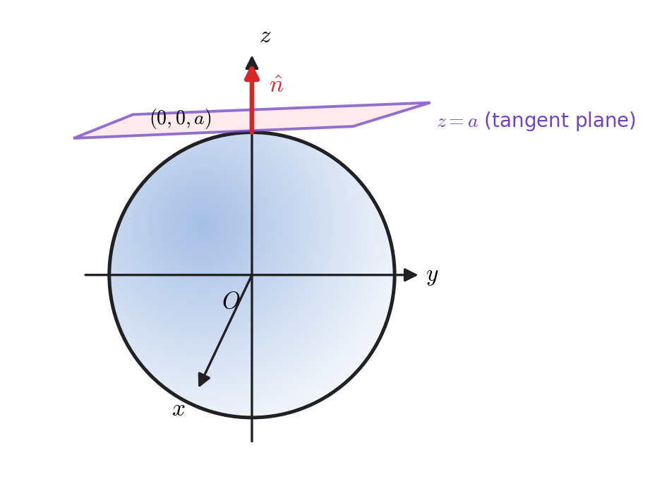
The tangent plane and the normal line to the sphere at the point considered.
Figure 6.4. The tangent plane and the normal line to the sphere at the point considered.
Theorem - Important Properties of the Gradient
  1. \(\vec{\nabla}(\phi+\psi)=\vec{\nabla}\phi+\vec{\nabla}\psi.\)

  2. \(\vec{\nabla}(m\phi)=m\vec{\nabla}\phi+\phi\vec{\nabla} m.\)

  3. \(\vec{\nabla}(\phi\psi)=\phi\vec{\nabla}\psi+\psi\vec{\nabla}\phi.\)

6.5Expressions Involving \(\vec{\nabla}\)

The differential operator

\begin{equation} \vec{\nabla} = \hat{i}\frac{\partial}{\partial x} + \hat{j}\frac{\partial}{\partial y} + \hat{k}\frac{\partial}{\partial z} \end{equation}

acts on scalar and vector fields in several useful ways.

Gradient of a Scalar Field

For a scalar field \(\phi(x,y,z)\),

\begin{equation} \vec{\nabla}\phi = \frac{\partial \phi}{\partial x}\hat{i}+\frac{\partial \phi}{\partial y}\hat{j}+\frac{\partial \phi}{\partial z}\hat{k}. \end{equation}

It produces a vector field pointing in the direction of the greatest increase of \(\phi\).

Divergence of a Vector Field

Definition - Divergence

If \(\vec{A}=A_x\hat{i}+A_y\hat{j}+A_z\hat{k}\), the divergence of \(\vec{A}\) is the scalar quantity

\begin{equation} \boxed{\vec{\nabla}\cdot\vec{A} = \frac{\partial A_x}{\partial x}+\frac{\partial A_y}{\partial y}+\frac{\partial A_z}{\partial z}.} \end{equation}
Remark

Divergence measures the net outflow of the field from a point. A positive divergence indicates a source; a negative divergence, a sink.

Curl of a Vector Field

Definition - Curl

For \(\vec{A}=A_x\hat{i}+A_y\hat{j}+A_z\hat{k}\), the curl is the vector

\begin{equation} \boxed{ \vec{\nabla}\times\vec{A}= \begin{vmatrix} \hat{i}&\hat{j}&\hat{k}\\ \frac{\partial}{\partial x}&\frac{\partial}{\partial y}&\frac{\partial}{\partial z}\\ A_x&A_y&A_z \end{vmatrix} = \left(\frac{\partial A_z}{\partial y}-\frac{\partial A_y}{\partial z}\right)\hat{i} +\left(\frac{\partial A_x}{\partial z}-\frac{\partial A_z}{\partial x}\right)\hat{j} +\left(\frac{\partial A_y}{\partial x}-\frac{\partial A_x}{\partial y}\right)\hat{k}.} \end{equation}
Remark

The curl measures the rotation or circulation density of a vector field about a point.

Example - Divergence and Curl of

\(\displaystyle \vec{V}(x,y,z)=x\sin y\,\hat{i}+\cos y\,\hat{j}+xy\,\hat{k}.\)

Components: \(V_x=x\sin y,\; V_y=\cos y,\; V_z=xy.\)

Divergence.

\begin{equation} \vec{\nabla}\!\cdot\!\vec{V} =\frac{\partial V_x}{\partial x}+\frac{\partial V_y}{\partial y}+\frac{\partial V_z}{\partial z} =\underbrace{\sin y}_{\partial V_x/\partial x} +\underbrace{(-\sin y)}_{\partial V_y/\partial y} +\underbrace{0}_{\partial V_z/\partial z} =0. \end{equation}
\begin{equation} \boxed{\;\vec{\nabla}\!\cdot\!\vec{V}=0\;} \quad\text{(a solenoidal/incompressible field).} \end{equation}

Curl.

\begin{equation} \vec{\nabla}\!\times\!\vec{V} =\begin{vmatrix} \hat{i}&\hat{j}&\hat{k}\\ \frac{\partial}{\partial x}&\frac{\partial}{\partial y}&\frac{\partial}{\partial z}\\ x\sin y&\cos y&xy \end{vmatrix} =\Big(\frac{\partial V_z}{\partial y}-\frac{\partial V_y}{\partial z}\Big)\hat{i} +\Big(\frac{\partial V_x}{\partial z}-\frac{\partial V_z}{\partial x}\Big)\hat{j} +\Big(\frac{\partial V_y}{\partial x}-\frac{\partial V_x}{\partial y}\Big)\hat{k}. \end{equation}

Compute each term:

\begin{equation} \frac{\partial V_z}{\partial y}=x,\quad \frac{\partial V_y}{\partial z}=0,\qquad \frac{\partial V_x}{\partial z}=0,\quad \frac{\partial V_z}{\partial x}=y,\qquad \frac{\partial V_y}{\partial x}=0,\quad \frac{\partial V_x}{\partial y}=x\cos y. \end{equation}

Therefore,

\begin{equation} \boxed{\;\vec{\nabla}\!\times\!\vec{V}=x\,\hat{i}-y\,\hat{j}-x\cos y\,\hat{k}\;} \end{equation}

which is nonzero, indicating local rotational behavior whose strength varies with \(x\) and \(y\).

Example - Comparing Divergence and Curl in 2D Flows

Consider three two–dimensional vector fields in the \(xy\)–plane:

\begin{equation} \begin{aligned} (1)\;& \text{Field } \vec{A} &: &\quad \vec{A} = kx\,\hat{i} + ky\,\hat{j} \quad &\text{(Pure Divergence)} \\[4pt] (2)\;& \text{Field } \vec{B} &: &\quad \vec{B} = -\omega y\,\hat{i} + \omega x\,\hat{j} \quad &\text{(Pure Curl / Rotation)} \\[4pt] (3)\;& \text{Field } \vec{A} + \vec{B} &: &\quad (kx - \omega y)\,\hat{i} + (ky + \omega x)\,\hat{j} \quad &\text{(Combined / Spiral Flow)} \end{aligned} \end{equation}

(a) Divergence

\begin{equation} \begin{aligned} \vec{\nabla}\cdot\vec{A} &= \frac{\partial A_x}{\partial x} + \frac{\partial A_y}{\partial y} = k + k = 2k, \\[4pt] \vec{\nabla}\cdot\vec{B} &= \frac{\partial B_x}{\partial x} + \frac{\partial B_y}{\partial y} = 0 + 0 = 0, \\[4pt] \vec{\nabla}\cdot(\vec{A}+\vec{B}) &= 2k. \end{aligned} \end{equation}

Thus, \(\vec{A}\) and \(\vec{A}+\vec{B}\) represent fields with a uniform outward expansion (a source flow), while \(\vec{B}\) has zero divergence — a purely rotational flow.

(b) Curl

In two dimensions, only the \(z\)–component of the curl is nonzero:

\begin{equation} (\vec{\nabla}\times\vec{A})_z = \frac{\partial A_y}{\partial x} - \frac{\partial A_x}{\partial y}. \end{equation}

Hence,

\begin{equation} \begin{aligned} (\vec{\nabla}\times\vec{A})_z &= 0, \\[4pt] (\vec{\nabla}\times\vec{B})_z &= 2\omega, \\[4pt] (\vec{\nabla}\times(\vec{A}+\vec{B}))_z &= 2\omega. \end{aligned} \end{equation}

(c) Physical Interpretation

  • \(\vec{A}\): Field lines radiate outward from the origin — a pure source field. \(\vec{\nabla}\cdot\vec{A} > 0\), \(\vec{\nabla}\times\vec{A} = 0.\)

  • \(\vec{B}\): Field lines form closed circles — a pure rotational (vortex) field. \(\vec{\nabla}\cdot\vec{B} = 0\), \(\vec{\nabla}\times\vec{B} \neq 0.\)

  • \(\vec{A}+\vec{B}\): Field lines spiral outward — a combination of source and rotation. Both divergence and curl are nonzero, producing a spiral flow.
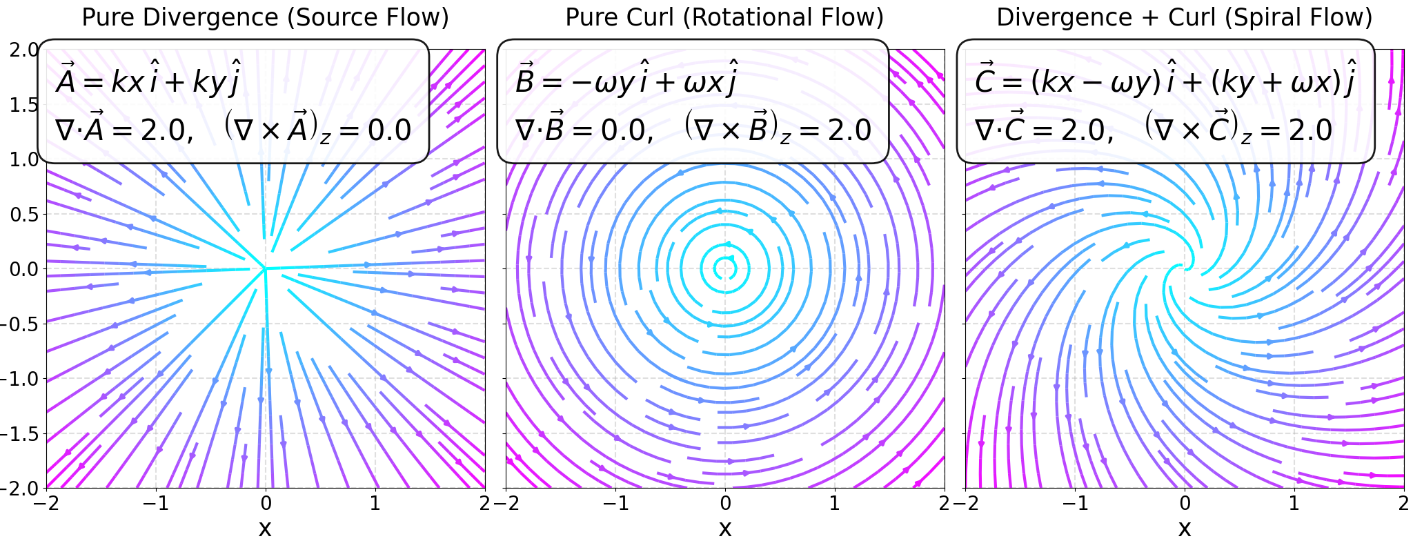
Field lines of A, of B, and of their sum: a pure source, a pure rotation, and the spiral flow that has both a divergence and a curl.
Figure 6.5. Field lines of \(\vec{A}\), of \(\vec{B}\), and of their sum: a pure source, a pure rotation, and the spiral flow that has both a divergence and a curl.

Visualization \(k=1\) and \(\omega=1 \)

  • Left: Pure source — arrows radiate outward uniformly.

  • Middle: Pure rotation — arrows circle around the origin.

  • Right: Spiral flow — arrows spiral outward, combining rotation and expansion.

This example clearly shows that:

  • Divergence quantifies the presence of sources or sinks.

  • Curl quantifies the local rotation of the field.

Example

Consider a rigid body rotating about the \(z\)-axis with a constant angular velocity \(\vec{\omega} = \omega\,\hat{k}\). Let the position vector of a point in the body be

\begin{equation} \vec{r} = x\,\hat{i} + y\,\hat{j} + z\,\hat{k}. \end{equation}

Then, the velocity field of the rotating body is given by

\begin{equation} \boxed{\;\vec{V} = \vec{\omega} \times \vec{r}\;} \end{equation}

or explicitly

\begin{equation} \vec{V} = \omega\,\hat{k} \times (x\,\hat{i} + y\,\hat{j} + z\,\hat{k}) = (-\omega y)\,\hat{i} + (\omega x)\,\hat{j} + 0\,\hat{k}. \end{equation}

Compute the curl:

\begin{equation} \vec{\nabla} \times \vec{V} = \begin{vmatrix} \hat{i} & \hat{j} & \hat{k}\\ \frac{\partial}{\partial x} & \frac{\partial}{\partial y} & \frac{\partial}{\partial z}\\ -\omega y & \omega x & 0 \end{vmatrix}. \end{equation}

Expanding the determinant:

\begin{equation} \vec{\nabla} \times \vec{V} = \left(0-0\right)\hat{i} - \left(0-0\right)\hat{j} + \left(\frac{\partial (\omega x)}{\partial x} - \frac{\partial (-\omega y)}{\partial y}\right)\hat{k}. \end{equation}

Simplify:

\begin{equation} \boxed{\;\vec{\nabla} \times \vec{V} = 2\omega\,\hat{k} = 2\,\vec{\omega}.\;} \end{equation}

Physical Meaning: For a rigid body, the curl of the velocity field equals twice the angular velocity vector:

\begin{equation} \vec{\nabla}\times\vec{V} = 2\vec{\omega}. \end{equation}

Thus, the curl measures the local rotational motion of the field.

Definition - Laplacian Operator

The Laplacian of a scalar field \(f(x,y,z)\) is defined as the divergence of its gradient:

\begin{equation} \boxed{ \nabla^2 f = \vec{\nabla}\cdot(\vec{\nabla} f). } \end{equation}

In Cartesian coordinates,

\begin{equation} \nabla^2 f = \frac{\partial^{2} f}{\partial x^{2}} + \frac{\partial^{2} f}{\partial y^{2}} + \frac{\partial^{2} f}{\partial z^{2}}. \end{equation}
Example - Laplacian of

\(\displaystyle f(x,y,z)=x^{3}-3xy^{2}+y^{3}\).

We use the Cartesian definition \(\displaystyle \nabla^{2}f=\frac{\partial^{2} f}{\partial x^{2}}+\frac{\partial^{2} f}{\partial y^{2}}+\frac{\partial^{2} f}{\partial z^{2}}\).

First derivatives:

\begin{equation} \frac{\partial f}{\partial x}=3x^{2}-3y^{2}, \qquad \frac{\partial f}{\partial y}=-6xy+3y^{2}, \qquad \frac{\partial f}{\partial z}=0. \end{equation}

Second derivatives:

\begin{equation} \frac{\partial^{2} f}{\partial x^{2}}=6x, \qquad \frac{\partial^{2} f}{\partial y^{2}}=-6x+6y, \qquad \frac{\partial^{2} f}{\partial z^{2}}=0. \end{equation}

Laplacian:

\begin{equation} \boxed{\;\nabla^{2} f = \left(6x\right)+\left(-6x+6y\right)+0 = 6y.\;} \end{equation}

Useful Vector Identities

Theorem - Common Vector Identities
  1. \(\vec{\nabla}\cdot(\vec{\nabla}\times\vec{A}) = 0.\) Physical meaning: This identity states that the divergence of a curl is always zero. In physical terms, a rotational (circulating) field such as a magnetic field has no net source or sink. For example, \(\vec{\nabla}\cdot\vec{B}=0\) in Maxwell’s equations expresses that there are no magnetic monopoles.

  2. \(\vec{\nabla}\times(\vec{\nabla}\phi) = \vec{0}.\) Physical meaning: This states that the curl of a gradient is always zero. It means that any field derived from a scalar potential (such as the electrostatic field \(\vec{E} = -\vec{\nabla}V\)) is irrotational—it has no circulation or rotational component.

  3. \(\vec{\nabla}\cdot(\phi\vec{A}) = \phi\,(\vec{\nabla}\cdot\vec{A}) + \vec{\nabla}\phi\cdot\vec{A}.\)

  4. \(\vec{\nabla}\times(\phi\vec{A}) = \phi\,(\vec{\nabla}\times\vec{A}) + (\vec{\nabla}\phi)\times\vec{A}.\)

  5. \(\vec{\nabla}\cdot(\vec{A}\times\vec{B}) = \vec{B}\cdot(\vec{\nabla}\times\vec{A}) - \vec{A}\cdot(\vec{\nabla}\times\vec{B}).\)

  6. \(\vec{\nabla}\times(\vec{\nabla}\times\vec{A}) = \vec{\nabla}(\vec{\nabla}\cdot\vec{A}) - \nabla^2\vec{A}.\)

Vector Differential Operators in a General Orthogonal Curvilinear Coordinate System

In many physical problems, Cartesian coordinates \((x,y,z)\) are not always the most convenient choice. We often use other coordinate systems such as cylindrical \((\rho,\phi,z)\) or spherical \((r,\theta,\phi)\), which are examples of orthogonal curvilinear coordinates.

Definition - Orthogonal Curvilinear Coordinates

Let a point in space be described by three parameters \((u_1,u_2,u_3)\), related to Cartesian coordinates by

\begin{equation} x = x(u_1,u_2,u_3), \qquad y = y(u_1,u_2,u_3), \qquad z = z(u_1,u_2,u_3). \end{equation}

The coordinate system is called orthogonal if the coordinate lines intersect at right angles everywhere.

At each point, define:

  • \(\hat{u}_1, \hat{u}_2, \hat{u}_3\): unit vectors tangent to the coordinate lines \(u_1, u_2, u_3\);

  • \(h_1, h_2, h_3\): scale factors (or metric coefficients) defined by

    \begin{equation} h_i = \left|\frac{\partial \vec{r}}{\partial u_i}\right|, \qquad (i=1,2,3), \end{equation}

    where \(\vec{r} = x\,\hat{i} + y\,\hat{j} + z\,\hat{k}\) is the position vector.

Then, the differential displacement is

\begin{equation} \boxed{ d\vec{r} = h_1\,\hat{u}_1\,du_1 + h_2\,\hat{u}_2\,du_2 + h_3\,\hat{u}_3\,du_3. } \end{equation}
Theorem - Gradient in Orthogonal Coordinates

For any scalar field \(f(u_1,u_2,u_3)\),

\begin{equation} \boxed{ \vec{\nabla} f = \hat{u}_1\,\frac{1}{h_1}\frac{\partial f}{\partial u_1} + \hat{u}_2\,\frac{1}{h_2}\frac{\partial f}{\partial u_2} + \hat{u}_3\,\frac{1}{h_3}\frac{\partial f}{\partial u_3}. } \end{equation}

This operator gives the rate and direction of maximum change of \(f\) in any orthogonal coordinate system.

Theorem - Divergence in Orthogonal Coordinates

For a vector field \(\vec{A} = A_1\,\hat{u}_1 + A_2\,\hat{u}_2 + A_3\,\hat{u}_3,\)

\begin{equation} \boxed{ \vec{\nabla}\cdot\vec{A} = \frac{1}{h_1h_2h_3}\! \left[ \frac{\partial}{\partial u_1}\!\big(h_2h_3A_1\big) + \frac{\partial}{\partial u_2}\!\big(h_3h_1A_2\big) + \frac{\partial}{\partial u_3}\!\big(h_1h_2A_3\big) \right]. } \end{equation}

This measures the net outflow per unit volume of the field \(\vec{A}\) from an infinitesimal region.

Theorem - Curl in Orthogonal Coordinates

For the same vector field \(\vec{A} = A_1\,\hat{u}_1 + A_2\,\hat{u}_2 + A_3\,\hat{u}_3,\)

\begin{equation} \boxed{ \vec{\nabla}\times\vec{A} = \frac{1}{h_1h_2h_3} \begin{vmatrix} h_1\hat{u}_1 & h_2\hat{u}_2 & h_3\hat{u}_3 \\[4pt] \frac{\partial}{\partial u_1} & \frac{\partial}{\partial u_2} & \frac{\partial}{\partial u_3} \\[4pt] h_1A_1 & h_2A_2 & h_3A_3 \end{vmatrix}. } \end{equation}

This represents the local rotation or circulation of the vector field \(\vec{A}\).

Theorem - Laplacian in Orthogonal Coordinates

The Laplacian of a scalar function \(f(u_1,u_2,u_3)\) is given by

\begin{equation} \boxed{ \nabla^2 f = \frac{1}{h_1h_2h_3} \left[ \frac{\partial}{\partial u_1}\!\left(\frac{h_2h_3}{h_1}\frac{\partial f}{\partial u_1}\right) + \frac{\partial}{\partial u_2}\!\left(\frac{h_3h_1}{h_2}\frac{\partial f}{\partial u_2}\right) + \frac{\partial}{\partial u_3}\!\left(\frac{h_1h_2}{h_3}\frac{\partial f}{\partial u_3}\right) \right]. } \end{equation}

It appears frequently in physics, for example in Poisson’s equation, the heat equation, and the Schrödinger equation.

Vector Differential Operators in Common Coordinate Systems

In vector calculus, the four most fundamental vector differential operators are:

\begin{equation} \text{Gradient: } \vec{\nabla} f, \qquad \text{Divergence: } \vec{\nabla}\cdot\vec{A}, \qquad \text{Curl: } \vec{\nabla}\times\vec{A}, \qquad \text{Laplacian: } \nabla^2 f = \vec{\nabla}\cdot(\vec{\nabla}f). \end{equation}

These operators describe spatial variation of scalar and vector fields, and their expressions depend on the coordinate system and corresponding unit vectors.

1) Cartesian Coordinates \((x, y, z)\)

\begin{align*} d\vec{r} &= \hat{i}\,dx + \hat{j}\,dy + \hat{k}\,dz, \\ (h_1,h_2,h_3) &= (1,1,1), \qquad (\hat{u}_1,\hat{u}_2,\hat{u}_3) = (\hat{i},\hat{j},\hat{k}). \end{align*}
\begin{equation} \boxed{ \begin{aligned} \text{Gradient:}\quad & \vec{\nabla}f = \hat{i}\frac{\partial f}{\partial x} + \hat{j}\frac{\partial f}{\partial y} + \hat{k}\frac{\partial f}{\partial z}, \\[4pt] \text{Divergence:}\quad & \vec{\nabla}\cdot\vec{A} = \frac{\partial A_x}{\partial x} + \frac{\partial A_y}{\partial y} + \frac{\partial A_z}{\partial z}, \\[4pt] \text{Curl:}\quad & \vec{\nabla}\times\vec{A} = \begin{vmatrix} \hat{i} & \hat{j} & \hat{k}\\ \frac{\partial}{\partial x} & \frac{\partial}{\partial y} & \frac{\partial}{\partial z}\\ A_x & A_y & A_z \end{vmatrix}, \\[4pt] \text{Laplacian:}\quad & \nabla^2 f = \frac{\partial^{2} f}{\partial x^{2}} + \frac{\partial^{2} f}{\partial y^{2}} + \frac{\partial^{2} f}{\partial z^{2}}. \end{aligned} } \end{equation}

2) Cylindrical Coordinates \((\rho, \phi, z)\)

\begin{align*} d\vec{r} &= \hat{\rho}\,d\rho + \rho\,\hat{\phi}\,d\phi + \hat{z}\,dz, \\ (h_1,h_2,h_3) &= (1,\rho,1), \qquad (\hat{u}_1,\hat{u}_2,\hat{u}_3) = (\hat{\rho},\hat{\phi},\hat{z}). \end{align*}

The unit vectors are related to the Cartesian basis by:

\begin{equation} \hat{\rho} = \cos\phi\,\hat{i} + \sin\phi\,\hat{j}, \qquad \hat{\phi} = -\sin\phi\,\hat{i} + \cos\phi\,\hat{j}, \qquad \hat{z} = \hat{k}. \end{equation}
\begin{equation} \boxed{ \begin{aligned} \text{Gradient:}\quad & \vec{\nabla}f = \hat{\rho}\,\frac{\partial f}{\partial \rho} + \frac{1}{\rho}\,\hat{\phi}\,\frac{\partial f}{\partial \phi} + \hat{z}\,\frac{\partial f}{\partial z}, \\[4pt] \text{Divergence:}\quad & \vec{\nabla}\cdot\vec{A} = \frac{1}{\rho}\,\frac{\partial}{\partial \rho}\!\big(\rho A_\rho\big) + \frac{1}{\rho}\,\frac{\partial A_\phi}{\partial \phi} + \frac{\partial A_z}{\partial z}, \\[4pt] \text{Curl:}\quad & \vec{\nabla}\times\vec{A} = \frac{1}{\rho} \begin{vmatrix} \hat{\rho} & \rho\hat{\phi} & \hat{z}\\ \frac{\partial}{\partial \rho} & \frac{\partial}{\partial \phi} & \frac{\partial}{\partial z}\\ A_\rho & \rho A_\phi & A_z \end{vmatrix}, \\[4pt] \text{Laplacian:}\quad & \nabla^2 f = \frac{1}{\rho}\,\frac{\partial}{\partial \rho}\!\left(\rho\,\frac{\partial f}{\partial \rho}\right) + \frac{1}{\rho^2}\,\frac{\partial^{2} f}{\partial \phi^{2}} + \frac{\partial^{2} f}{\partial z^{2}}. \end{aligned} } \end{equation}

3) Spherical Coordinates \((r, \theta, \phi)\)

\begin{align*} d\vec{r} &= \hat{r}\,dr + r\,\hat{\theta}\,d\theta + r\sin\theta\,\hat{\phi}\,d\phi, \\ (h_1,h_2,h_3) &= (1,r,r\sin\theta), \qquad (\hat{u}_1,\hat{u}_2,\hat{u}_3) = (\hat{r},\hat{\theta},\hat{\phi}). \end{align*}

The spherical unit vectors in terms of Cartesian components are:

\begin{equation} \begin{aligned} \hat{r} &= \sin\theta\cos\phi\,\hat{i} + \sin\theta\sin\phi\,\hat{j} + \cos\theta\,\hat{k}, \\ \hat{\theta} &= \cos\theta\cos\phi\,\hat{i} + \cos\theta\sin\phi\,\hat{j} - \sin\theta\,\hat{k}, \\ \hat{\phi} &= -\sin\phi\,\hat{i} + \cos\phi\,\hat{j}. \end{aligned} \end{equation}
\begin{equation} \boxed{ \begin{aligned} \text{Gradient:}\quad & \vec{\nabla}f = \hat{r}\,\frac{\partial f}{\partial r} + \frac{1}{r}\,\hat{\theta}\,\frac{\partial f}{\partial \theta} + \frac{1}{r\sin\theta}\,\hat{\phi}\,\frac{\partial f}{\partial \phi}, \\[4pt] \text{Divergence:}\quad & \vec{\nabla}\cdot\vec{A} = \frac{1}{r^2}\,\frac{\partial}{\partial r}\!\big(r^2A_r\big) + \frac{1}{r\sin\theta}\,\frac{\partial}{\partial \theta}\!\big(\sin\theta\,A_\theta\big) + \frac{1}{r\sin\theta}\,\frac{\partial A_\phi}{\partial \phi}, \\[4pt] \text{Curl:}\quad & \vec{\nabla}\times\vec{A} = \frac{1}{r^2\sin\theta} \begin{vmatrix} \hat{r} & r\hat{\theta} & r\sin\theta\,\hat{\phi}\\ \frac{\partial}{\partial r} & \frac{\partial}{\partial \theta} & \frac{\partial}{\partial \phi}\\ A_r & rA_\theta & r\sin\theta\,A_\phi \end{vmatrix}, \\[4pt] \text{Laplacian:}\quad & \nabla^2 f = \frac{1}{r^2}\,\frac{\partial}{\partial r}\!\left(r^2\,\frac{\partial f}{\partial r}\right) + \frac{1}{r^2\sin\theta}\,\frac{\partial}{\partial \theta}\!\left(\sin\theta\,\frac{\partial f}{\partial \theta}\right) + \frac{1}{r^2\sin^2\theta}\,\frac{\partial^{2} f}{\partial \phi^{2}}. \end{aligned} } \end{equation}

6.6Maxwell’s Equations in Vacuum

In differential form, Maxwell’s equations describe the behavior of electric and magnetic fields in space and time. They connect the electric field \(\vec{E}\), magnetic field \(\vec{B}\), charge density \(\rho\), and current density \(\vec{J}\).

Theorem - Maxwell’s Equations (Differential Form in Vacuum with Sources)
\begin{equation} \begin{aligned} \text{(1) Gauss’s Law:} &\quad \vec{\nabla}\cdot\vec{E} = \frac{\rho_f}{\epsilon_0}, \\[4pt] \text{(2) Gauss’s Law for Magnetism:} &\quad \vec{\nabla}\cdot\vec{B} = 0, \\[4pt] \text{(3) Faraday’s Law of Induction:} &\quad \vec{\nabla}\times\vec{E} = -\,\frac{\partial \vec{B}}{\partial t}, \\[4pt] \text{(4) Ampère–Maxwell Law:} &\quad \vec{\nabla}\times\vec{B} = \mu_0\,\vec{J}_f + \mu_0\epsilon_0\,\frac{\partial \vec{E}}{\partial t}. \end{aligned} \end{equation}
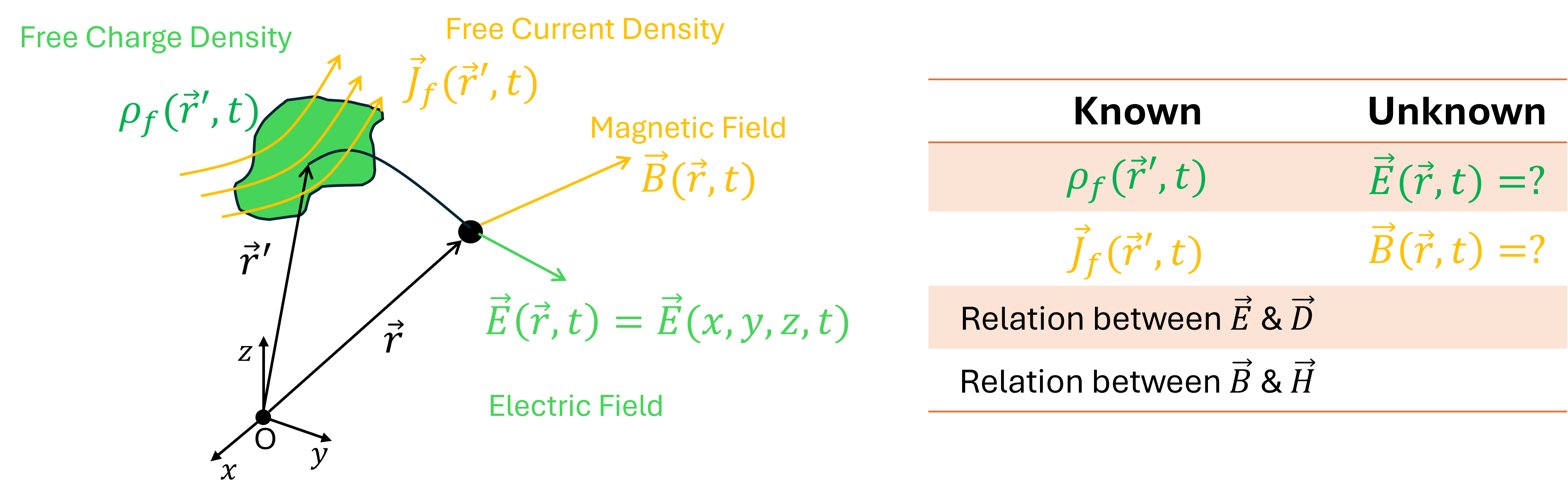
What Maxwell's equations relate. The free charge density f(r\,&#x27;,t) and free current density Jf(r\,&#x27;,t) at the source point are given; the fields E(r,t) and B(r,t) at the field point are what is to be found.
Figure 6.6. What Maxwell's equations relate. The free charge density \(\rho_f(\vec{r}\,',t)\) and free current density \(\vec{J}_f(\vec{r}\,',t)\) at the source point are given; the fields \(\vec{E}(\vec{r},t)\) and \(\vec{B}(\vec{r},t)\) at the field point are what is to be found.

Physical Meaning of Each Equation

  1. Gauss’s Law: \(\displaystyle \vec{\nabla}\cdot\vec{E} = \frac{\rho_f}{\epsilon_0}\)

    • The divergence of the electric field gives the local charge density.

    • Positive charges are sources of electric field lines, negative charges are sinks.

  2. Gauss’s Law for Magnetism: \(\displaystyle \vec{\nabla}\cdot\vec{B} = 0\)

    • Magnetic field lines are always closed loops; there are no magnetic monopoles.

    • The field has no divergence—no “beginning” or “end.”

  3. Faraday’s Law: \(\displaystyle \vec{\nabla}\times\vec{E} = -\frac{\partial \vec{B}}{\partial t}\)

    • A time-varying magnetic field induces a circulating electric field.

    • The curl of \(\vec{E}\) represents the tendency of \(\vec{E}\) to form closed loops.

    • This is the principle behind electromagnetic induction.

  4. Ampère–Maxwell Law: \(\displaystyle \vec{\nabla}\times\vec{B} = \mu_0\vec{J}_f + \mu_0\epsilon_0\frac{\partial \vec{E}}{\partial t}\)

    • A circulating magnetic field is produced by electric currents \(\vec{J}\) and by changing electric fields \(\frac{\partial \vec{E}}{\partial t}\).

    • The second term (\(\mu_0\epsilon_0\frac{\partial \vec{E}}{\partial t}\)) is the displacement current density, introduced by Maxwell to ensure charge conservation.
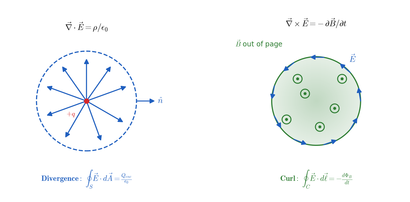
Divergence and curl side by side. Left: the flux of E out of a closed surface enclosing a charge +q, which integrates to Gauss's law. Right: the circulation of E around a loop threaded by a changing B, which integrates to Faraday's law.
Figure 6.7. Divergence and curl side by side. Left: the flux of \(\vec{E}\) out of a closed surface enclosing a charge \(+q\), which integrates to Gauss's law. Right: the circulation of \(\vec{E}\) around a loop threaded by a changing \(\vec{B}\), which integrates to Faraday's law.

Derivation of the Electromagnetic Wave Equation

We now derive how Maxwell’s equations predict that changing electric and magnetic fields propagate as waves in vacuum. In Vacuum (no charges or currents): \(\rho_f = 0\), \(\vec{J}_f = 0.\) Then Maxwell’s equations become:

\begin{equation} \boxed{ \begin{aligned} \vec{\nabla}\cdot\vec{E} &= 0, & \vec{\nabla}\cdot\vec{B} &= 0, \\[4pt] \vec{\nabla}\times\vec{E} &= -\frac{\partial \vec{B}}{\partial t}, & \vec{\nabla}\times\vec{B} &= \mu_0\epsilon_0\,\frac{\partial \vec{E}}{\partial t}. \end{aligned} } \end{equation}

Derivation of the wave equation.

Take the curl of Faraday’s law:

\begin{equation} \vec{\nabla} \times (\vec{\nabla} \times \vec{E}) = -\,\frac{\partial}{\partial t}\!\big(\vec{\nabla} \times \vec{B}\big). \end{equation}

Substitute \(\vec{\nabla}\times\vec{B} = \mu_0\epsilon_0\,\frac{\partial \vec{E}}{\partial t}\):

\begin{equation} \vec{\nabla}\times(\vec{\nabla}\times\vec{E}) = -\,\mu_0\epsilon_0\,\frac{\partial^{2} \vec{E}}{\partial t^{2}}. \end{equation}

Using the vector identity

\begin{equation} \vec{\nabla}\times(\vec{\nabla}\times\vec{E}) = \vec{\nabla}(\vec{\nabla}\cdot\vec{E}) - \nabla^2\vec{E}, \end{equation}

and since \(\vec{\nabla}\cdot\vec{E}=0\) in vacuum, we obtain:

\begin{equation} \boxed{ \nabla^2\vec{E} = \mu_0\epsilon_0\,\frac{\partial^{2} \vec{E}}{\partial t^{2}}. } \end{equation}

Similarly, taking the curl of \(\vec{\nabla}\times\vec{B} = \mu_0\epsilon_0\,\frac{\partial \vec{E}}{\partial t}\) gives:

\begin{equation} \boxed{ \nabla^2\vec{B} = \mu_0\epsilon_0\,\frac{\partial^{2} \vec{B}}{\partial t^{2}}. } \end{equation}

These are wave equations for \(\vec{E}\) and \(\vec{B}\), describing electromagnetic waves propagating through space.

The wave speed.

Comparing with the standard wave equation \(\nabla^2 u = \dfrac{1}{v^{2}}\frac{\partial^{2} u}{\partial t^{2}}\), whose solutions travel at speed \(v\), we can read off the speed of an electromagnetic wave:

\begin{equation} \frac{1}{v^{2}} = \mu_0\epsilon_0 \qquad\Longrightarrow\qquad \boxed{\,v = \frac{1}{\sqrt{\mu_0\epsilon_0}} \equiv c\,}. \end{equation}

Substituting the measured constants \(\mu_0 = 4\pi\times10^{-7}\ \mathrm{T\,m/A}\) and \(\epsilon_0 = 8.85\times10^{-12}\ \mathrm{C^2/(N\,m^2)}\) gives \(c \approx 3.00\times10^{8}\ \mathrm{m/s}\) — the measured speed of light. This is the historical significance of the calculation: two constants obtained from benchtop experiments on static electricity and on magnets combine to give the speed of light, which is what identified light itself as an electromagnetic wave.
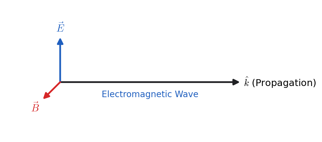
An electromagnetic wave: E and B oscillate perpendicular to each other and to the direction of travel.
Figure 6.8. An electromagnetic wave: \(\vec{E}\) and \(\vec{B}\) oscillate perpendicular to each other and to the direction of travel.

6.7Vector Integrals

In vector calculus, integrals of scalar or vector functions can be defined over curves, surfaces, or volumes. These are classified as:

\begin{equation} \text{Line Integrals}, \qquad \text{Surface Integrals}, \qquad \text{and Volume Integrals.} \end{equation}

6.7.1Line Integrals

We may encounter three types of line integrals along a curve \( C \):

\begin{equation} \int_C \phi\, d\vec{r}, \qquad \int_C \vec{A}\cdot d\vec{r}, \qquad \text{and} \qquad \int_C \vec{A}\times d\vec{r}. \end{equation}
Example

Evaluate

\begin{equation} I = \int_C \vec{F}\cdot d\vec{r}, \qquad \text{where } \vec{F} = (x+y)\,\hat{i} + (y-x)\,\hat{j}, \end{equation}

along each of the following paths.

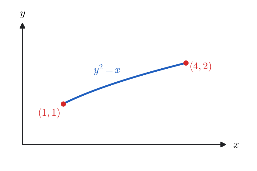
(i) Parabolic path \(y^2 = x\) from \((1,1)\) to \((4,2)\).

Step 1. Express \(d\vec{r}\).

Since \(x = y^2\), we have

\begin{equation} d\vec{r} = dx\,\hat{i} + dy\,\hat{j} = (2y\,dy)\,\hat{i} + dy\,\hat{j}. \end{equation}

Step 2. Compute \(\vec{F}\cdot d\vec{r}\).

\begin{equation} \vec{F}\cdot d\vec{r} = (x+y)\,dx + (y-x)\,dy = (y^2+y)(2y\,dy) + (y - y^2)\,dy = (2y^3 + y^2 + y)\,dy. \end{equation}

Step 3. Integrate from \(y=1\) to \(y=2\).

\begin{equation} I = \int_1^2 (2y^3 + y^2 + y)\,dy = \left[\frac{y^4}{2} + \frac{y^3}{3} + \frac{y^2}{2}\right]_1^2 = \frac{34}{3}. \end{equation}
The path of integration: the parabola y^2=x from (1,1) to (4,2).
Figure 6.9. The path of integration: the parabola \(y^{2}=x\) from \((1,1)\) to \((4,2)\).

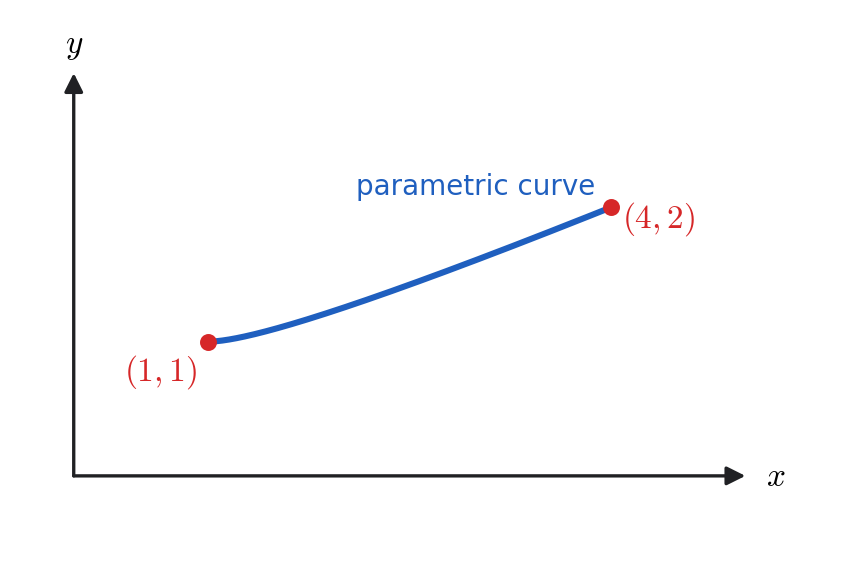
(ii) Parametric curve \(x=2u^2+u+1\), \(y=1+u^2\) from \((1,1)\) to \((4,2)\).

Step 1. Express \(d\vec{r}\).

\begin{equation} d\vec{r} = dx\,\hat{i} + dy\,\hat{j} = (4u+1)\,du\,\hat{i} + (2u)\,du\,\hat{j}. \end{equation}

Step 2. Compute \(\vec{F}\cdot d\vec{r}\).

\begin{equation} \vec{F}\cdot d\vec{r} = (x+y)\,dx + (y-x)\,dy. \end{equation}

Substitute \(x=2u^2+u+1\), \(y=1+u^2\):

\begin{equation} x+y = 3u^2 + u + 2, \qquad y-x = -u^2 - u. \end{equation}

Thus,

\begin{equation} \vec{F}\cdot d\vec{r} = (3u^2 + u + 2)(4u+1)\,du - (u^2 + u)(2u)\,du . \end{equation}

Expanding each product separately,

\begin{equation} (3u^2 + u + 2)(4u+1) = 12u^3 + 7u^2 + 9u + 2, \qquad (u^2+u)(2u) = 2u^3 + 2u^2, \end{equation}

so that

\begin{equation} \vec{F}\cdot d\vec{r} = \big(12u^3 + 7u^2 + 9u + 2 - 2u^3 - 2u^2\big)\,du = (10u^3 + 5u^2 + 9u + 2)\,du. \end{equation}

Step 3. Integrate from \(u=0\) to \(u=1\).

\begin{equation} I = \int_0^1 (10u^3 + 5u^2 + 9u + 2)\,du = \left[\frac{10u^4}{4} + \frac{5u^3}{3} + \frac{9u^2}{2} + 2u\right]_0^1 = \frac{5}{2} + \frac{5}{3} + \frac{9}{2} + 2 = \frac{32}{3}. \end{equation}
The same two endpoints joined by a parametric curve from (1,1) to (4,2).
Figure 6.10. The same two endpoints joined by a parametric curve from \((1,1)\) to \((4,2)\).

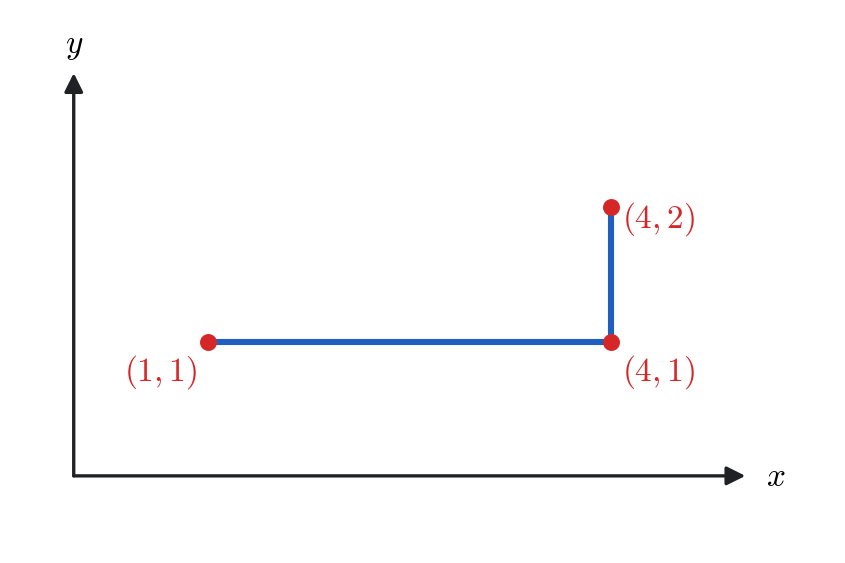
(iii) Piecewise linear path.

Segment 1: along \(y=1\) from \((1,1)\) to \((4,1)\).

\begin{equation} d\vec{r} = dx\,\hat{i} \quad (dy=0), \quad \vec{F}\cdot d\vec{r} = (x+y)\,dx = (x+1)\,dx. \end{equation}
\begin{equation} I_1 = \int_1^4 (x+1)\,dx = \left[\frac{x^2}{2}+x\right]_1^4 = \frac{21}{2}. \end{equation}

Segment 2: along \(x=4\) from \((4,1)\) to \((4,2)\).

\begin{equation} d\vec{r} = dy\,\hat{j} \quad (dx=0), \quad \vec{F}\cdot d\vec{r} = (y-x)\,dy = (y-4)\,dy. \end{equation}
\begin{equation} I_2 = \int_1^2 (y-4)\,dy = \left[\frac{y^2}{2}-4y\right]_1^2 = -\frac{5}{2}. \end{equation}

Total:

\begin{equation} I = I_1 + I_2 = \frac{21}{2} - \frac{5}{2} = 8. \end{equation}
The same two endpoints joined by a piecewise path: straight from (1,1) to (4,1), then straight up to (4,2).
Figure 6.11. The same two endpoints joined by a piecewise path: straight from \((1,1)\) to \((4,1)\), then straight up to \((4,2)\).
Remark - Observation

Although all three paths start and end at the same points, the resulting integrals differ:

\begin{equation} I_{\text{(i)}} = \frac{34}{3}, \qquad I_{\text{(ii)}} = \frac{32}{3}, \qquad I_{\text{(iii)}} = 8. \end{equation}

Therefore, \(\vec{F}\) is a non-conservative vector field, since \(\int_C \vec{F}\cdot d\vec{r}\) depends on the path taken.

Example

Evaluate the line integral

\begin{equation} I = \oint_C x\,dy, \end{equation}

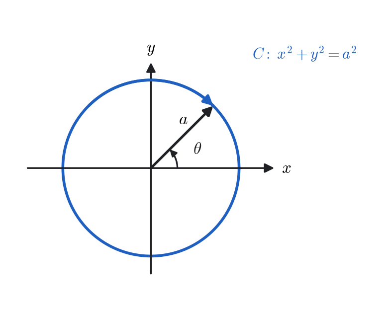
where \(C\) is the circle in the \(xy\)–plane defined by

\begin{equation} x^2 + y^2 = a^2, \qquad z = 0. \end{equation}

Solution.

This integral is very simple in polar coordinates.

\begin{equation} x = a\cos\theta, \qquad y = a\sin\theta, \qquad dy = a\cos\theta\,d\theta. \end{equation}
\begin{equation} I = \oint_C x\,dy = \int_0^{2\pi} a\cos\theta\,(a\cos\theta\,d\theta) = a^2\int_0^{2\pi}\cos^2\theta\,d\theta. \end{equation}

Using the trigonometric identity \(\cos^2\theta = \dfrac{1+\cos(2\theta)}{2}\),

\begin{equation} I = a^2\int_0^{2\pi}\frac{1+\cos(2\theta)}{2}\,d\theta = \frac{a^2}{2}\Big[\theta + \frac{\sin(2\theta)}{2}\Big]_0^{2\pi}. \end{equation}

Since \(\sin(2\pi)=0\),

\begin{equation} \boxed{\,I = \pi a^2.\,} \end{equation}
The circular contour of radius a, traversed once, for which I= a^2.
Figure 6.12. The circular contour of radius \(a\), traversed once, for which \(I=\pi a^{2}\).
Example - Compute the line integral
\begin{equation} I=\int_C \frac{x\,dy - y\,dx}{x^2+y^2} \end{equation}

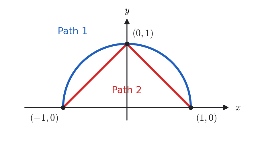
from \((-1,0)\) to \((1,0)\) along the two paths shown below.

The two paths from (-1,0) to (1,0) compared in this example.
Figure 6.13. The two paths from \((-1,0)\) to \((1,0)\) compared in this example.

We can write this integral as

\begin{equation} I=\int_C \vec{F}\cdot d\vec{r}, \qquad \text{where } \vec{F} = \frac{-y\,\hat{i} + x\,\hat{j}}{x^2 + y^2}, \end{equation}

along each of the following paths.

Path 1: upper semicircle of the unit circle

Use polar coordinates on the circle \(r=1\): \(x=\cos\theta,\ y=\sin\theta,\ dx=-\sin\theta\,d\theta,\ dy=\cos\theta\,d\theta,\ x^2+y^2=1.\)

\begin{equation} \frac{x\,dy-y\,dx}{x^2+y^2} =\cos\theta(\cos\theta\,d\theta)-\sin\theta(-\sin\theta\,d\theta) =\big(\cos^2\theta+\sin^2\theta\big)d\theta=d\theta. \end{equation}

Along the upper semicircle from \((-1,0)\) to \((1,0)\) we have \(\theta:\ \pi\to 0\). Hence

\begin{equation} \boxed{\,I_1=\int_{\pi}^{0} d\theta=-\pi.\,} \end{equation}

Path 2: two straight-line segments

Segment A.

From \((-1,0)\) to \((0,1)\) along \(y=x+1\). Then \(dy=dx\) and

\begin{equation} x\,dy-y\,dx = \big(x-(x+1)\big)\,dx = -\,dx,\qquad x^2+y^2 = x^2+(x+1)^2=2x^2+2x+1. \end{equation}

Thus

\begin{equation} I_A=\int_{-1}^{0}\frac{-\,dx}{2x^2+2x+1} =\int_{-1}^{0}\frac{-2\,dx}{(2x+1)^2+1} =-\Big[\arctan(2x+1)\Big]_{-1}^{0} =-\frac{\pi}{2}. \end{equation}

Segment B.

From \((0,1)\) to \((1,0)\) along \(y=1-x\). Then \(dy=-dx\) and

\begin{equation} x\,dy-y\,dx = \big(-x-(1-x)\big)\,dx = -\,dx,\qquad x^2+y^2 = x^2+(1-x)^2=2x^2-2x+1. \end{equation}

Hence

\begin{equation} I_B=\int_{0}^{1}\frac{-\,dx}{2x^2-2x+1} =\int_{0}^{1}\frac{-2\,dx}{(2x-1)^2+1} =-\Big[\arctan(2x-1)\Big]_{0}^{1} =-\frac{\pi}{2}. \end{equation}
\begin{equation} \boxed{\,I_2=I_A+I_B=-\frac{\pi}{2}-\frac{\pi}{2}=-\pi.\,} \end{equation}

6.7.2Conservative Fields

A force field \(\vec{F}\) is said to be conservative if the work done by it is independent of the path between two points:

\begin{equation} W = \int_C \vec{F}\cdot d\vec{r} \quad \text{is path independent.} \end{equation}

If \(W\) depends on the path, then \(\vec{F}\) is non-conservative, and energy is being dissipated (e.g., by friction).

Condition for a Conservative Field

A vector field \(\vec{F}\) is conservative if and only if

\begin{equation} \vec{\nabla}\times\vec{F} = \vec{0}. \end{equation}

In this case, \(\vec{F}\) can be expressed as the gradient of a scalar potential \(W(x,y,z)\):

\begin{equation} \vec{F} = \vec{\nabla}W = \hat{i}\,\frac{\partial W}{\partial x} + \hat{j}\,\frac{\partial W}{\partial y} + \hat{k}\,\frac{\partial W}{\partial z}. \end{equation}

Taking the curl of both sides:

\begin{equation} \vec{\nabla}\times\vec{F} = \vec{\nabla}\times(\vec{\nabla}W) = \vec{0}, \end{equation}

which confirms that \(\vec{F}\) is indeed conservative.

Work in Terms of Potential Function

If \(\vec{F} = \vec{\nabla}W\), then

\begin{equation} \vec{F}\cdot d\vec{r} = \vec{\nabla}W\cdot d\vec{r} = \frac{\partial W}{\partial x}\,dx + \frac{\partial W}{\partial y}\,dy + \frac{\partial W}{\partial z}\,dz = dW. \end{equation}

Hence,

\begin{equation} \int_A^B \vec{F}\cdot d\vec{r} = \int_A^B dW = W(B) - W(A). \end{equation}

The work done depends only on the values of \(W\) at the endpoints.

Potential Function

For a conservative field we have \(\vec{F} = \vec{\nabla}W\), where \(W\) is the work function. In physics it is conventional to work instead with the potential energy \(\Phi\), defined as the negative of the work function:

\begin{equation} \Phi = -\,W \quad \text{(scalar potential)}, \end{equation}

and therefore,

\begin{equation} \boxed{\vec{F} = -\,\vec{\nabla}\Phi.} \end{equation}

The sign is not arbitrary: with this definition the force points in the direction of decreasing potential, so a ball rolls downhill and a positive charge moves away from another positive charge. Work done by the field lowers the potential energy, \(W(B)-W(A) = -[\Phi(B)-\Phi(A)]\), which is what makes \(\Phi\) the quantity that adds to kinetic energy to give a conserved total. Both conventions appear in the literature; the sign of the gradient must be checked whenever a potential is quoted.

Example

Show that \(\vec{F}\) where \(\vec{F}=-\vec{\nabla}\phi\).

Given

\begin{equation} \vec{F}(x,y,z)= (2xy - z^{3})\,\hat{i}\;+\;x^{2}\,\hat{j}\;-\;(3xz^{2}+1)\,\hat{k}. \end{equation}

We will (i) verify \(\vec{\nabla}\times\vec{F}=\vec{0}\), (ii) find a scalar potential by component integration, and (iii) confirm the result by an explicit path integral from \((0,0,0)\) to \((x,y,z)\).

Step 1 — Check \(\vec{\nabla}\times\vec{F}=\vec{0}\) (conservative test).

\begin{equation} \vec{\nabla}\times\vec{F} = \begin{vmatrix} \hat{i}&\hat{j}&\hat{k}\\ \frac{\partial}{\partial x}&\frac{\partial}{\partial y}&\frac{\partial}{\partial z}\\ 2xy-z^3 & x^2 & -(3xz^2+1) \end{vmatrix}. \end{equation}

Compute components carefully:

\begin{equation} \begin{aligned} (\vec{\nabla}\times\vec{F})_x &= \frac{\partial}{\partial y}\!\big(-(3xz^2+1)\big)-\frac{\partial}{\partial z}\!\big(x^2\big) = 0-0=0,\\[4pt] (\vec{\nabla}\times\vec{F})_y &= \frac{\partial}{\partial z}\!\big(2xy-z^3\big)-\frac{\partial}{\partial x}\!\big(-(3xz^2+1)\big) = (-3z^2) - (-3z^2)=0,\\[4pt] (\vec{\nabla}\times\vec{F})_z &= \frac{\partial}{\partial x}\!\big(x^2\big)-\frac{\partial}{\partial y}\!\big(2xy-z^3\big) = (2x)-(2x)=0. \end{aligned} \end{equation}

Hence \(\vec{\nabla}\times\vec{F}=\vec{0}\). On a simply connected domain in \(\mathbb{R}^3\) (e.g. all of \(\mathbb{R}^3\)), this implies that \(\vec{F}\) is conservative.

Step 2 — Find the work function by component integration. We seek \(W\) with \(\vec{F}=\vec{\nabla}W\), so the three partial derivatives of \(W\) are the three components of \(\vec{F}\). Integrate the first one in \(x\), holding \(y\) and \(z\) fixed:

\begin{equation} \frac{\partial W}{\partial x} = 2xy - z^{3} \quad\Longrightarrow\quad W = x^{2}y - xz^{3} + f(y,z), \end{equation}

where the “constant” of integration may still depend on \(y\) and \(z\). Now impose the second component:

\begin{equation} \frac{\partial W}{\partial y} = x^{2} + \frac{\partial f}{\partial y} \stackrel{!}{=} x^{2} \quad\Longrightarrow\quad \frac{\partial f}{\partial y}=0, \end{equation}

so \(f\) depends on \(z\) alone, \(f=f(z)\). Finally impose the third component:

\begin{equation} \frac{\partial W}{\partial z} = -3xz^{2} + f'(z) \stackrel{!}{=} -(3xz^{2}+1) \quad\Longrightarrow\quad f'(z) = -1, \end{equation}

giving \(f(z) = -z + C\). Therefore

\begin{equation} \boxed{\,W = x^{2}y - xz^{3} - z + C\,}, \qquad \Phi = -W = -x^{2}y + xz^{3} + z + C'. \end{equation}

As a check, \(\vec{\nabla}W = (2xy-z^{3})\hat{i} + x^{2}\hat{j} - (3xz^{2}+1)\hat{k} = \vec{F}\).

Step 3 — Confirm by an explicit path integral. Because \(\vec{F}\) is conservative we may choose any convenient path from the origin to \((x,y,z)\). Take three straight segments along the axes in turn, and set \(C=0\) so that \(W(0,0,0)=0\).

Segment 1, from \((0,0,0)\) to \((x,0,0)\) with \(y=z=0\): here \(d\vec{r}=dx'\,\hat{i}\) and \(F_x = 2x'(0)-0^{3}=0\), so this segment contributes nothing.

Segment 2, from \((x,0,0)\) to \((x,y,0)\): here \(d\vec{r}=dy'\,\hat{j}\) and \(F_y = x^{2}\), which is constant along the segment, so

\begin{equation} \int_{0}^{y} x^{2}\,dy' = x^{2}y . \end{equation}

Segment 3, from \((x,y,0)\) to \((x,y,z)\): here \(d\vec{r}=dz'\,\hat{k}\) and \(F_z = -(3xz'^{2}+1)\), so

\begin{equation} -\int_{0}^{z} \big(3xz'^{2}+1\big)\,dz' = -\big(xz^{3} + z\big). \end{equation}

Adding the three contributions,

\begin{equation} W(x,y,z) = 0 + x^{2}y - xz^{3} - z, \end{equation}

which agrees with the result of Step 2.

Physical Examples of Line Integrals

Line integrals appear frequently in physics, where they often represent quantities such as work, circulation, or magnetic flux linkage.

Below are some important physical contexts where line integrals are used.

1. Work Done by a Force Field

\begin{equation} W = \int_C \vec{F}\cdot d\vec{r} \end{equation}

This represents the work done by a force \(\vec{F}\) in moving a particle along a path \(C\).

2. Electrostatic Potential Energy

The electrostatic potential energy gained by moving a charge \(q\) through an electric field \(\vec{E}\) along a path \(C\) is

\begin{equation} V = -\,q\int_C \vec{E}\cdot d\vec{r}. \end{equation}

The negative sign indicates that the electric field does work against the potential difference.

3. Ampère’s Law (Magnetostatics)

The circulation of the magnetic field around a closed loop \(C\) is proportional to the current \(I\) enclosed by that loop:

\begin{equation} \oint_C \vec{B}\cdot d\vec{r} = \mu_0 I. \end{equation}

This integral form of Ampère’s law relates magnetic fields to the steady currents that produce them.

4. Magnetic Force on a Current Loop

A current-carrying wire placed in a magnetic field \(\vec{B}\) experiences a magnetic force given by

\begin{equation} \vec{F} = I \oint_C d\vec{r} \times \vec{B}. \end{equation}

This expression gives the total force on a loop of current \(I\) in a magnetic field. Each element of the wire experiences an infinitesimal force \(d\vec{F} = I\,d\vec{r}\times\vec{B}\).

6.7.11Surface and Volume Integrals

Surface Integrals

A surface integral generalizes the concept of a line integral to a two-dimensional surface. For a surface \(\sigma\) with unit normal vector \(\hat{n}\) and differential area element \(d\vec{\sigma} = \hat{n}\,d\sigma\), we can define three common types of surface integrals:

\begin{equation} \int_{\sigma} \phi\, d\vec{\sigma}, \qquad \int_{\sigma} \vec{F}\cdot d\vec{\sigma}, \qquad \int_{\sigma} \vec{F}\times d\vec{\sigma}. \end{equation}

The most important and frequently encountered is

\begin{equation} \boxed{\Phi = \iint_{\sigma} \vec{F}\cdot d\vec{\sigma}}, \end{equation}

which represents the flux of the vector field \(\vec{F}\) through the surface \(S\). Physically, this measures how much of the field “flows” through \(S\). Only the normal component of \(\vec{F}\) contributes to the flux; tangential components make no contribution.
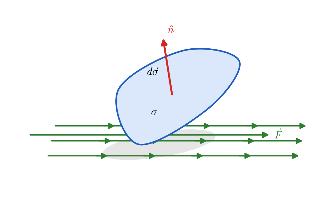
Flux through a surface: only the component of F along the normal crosses S, and the tangential component contributes nothing.
Figure 6.14. Flux through a surface: only the component of \(\vec{F}\) along the normal crosses \(S\), and the tangential component contributes nothing.

Volume Integrals

A volume integral extends the concept to three dimensions. For a scalar field \(\phi(x,y,z)\),

\begin{equation} \int_{\tau} \phi\, d\tau \end{equation}

represents the total accumulation of \(\phi\) over a volume \(V\).

For a vector field \(\vec{A} = A_x\,\hat{i} + A_y\,\hat{j} + A_z\,\hat{k}\),

\begin{equation} \int_{\tau} \vec{A}\, d\tau = \hat{i}\int_{\tau} A_x\, d\tau + \hat{j}\int_{\tau} A_y\, d\tau + \hat{k}\int_{\tau} A_z\, d\tau, \end{equation}

reducing the vector integral to a sum of scalar volume integrals over the components.

6.7.14Green’s Theorem in the Plane

The one–dimensional Fundamental Theorem of Calculus states:

\begin{equation} \int_a^b \frac{d f(t)}{d t}\,dt = f(b) - f(a), \end{equation}

relating the integral of a derivative over an interval to the function’s change at its endpoints. In two dimensions, a similar idea holds: the integral of derivatives over an area \(A\) corresponds to function values along its boundary \(C\). This reasoning leads directly to Green’s Theorem.

Theorem - Green’s Theorem

If \(P(x,y)\) and \(Q(x,y)\) have continuous first partial derivatives in a simply connected region \(A\) bounded by a positively oriented closed curve \(C\), then

\begin{equation} \boxed{ \oint_{\partial A} (P\,dx + Q\,dy) = \iint_A \left( \frac{\partial Q}{\partial x} - \frac{\partial P}{\partial y} \right) dx\,dy. } \end{equation}

Proof

Part I: the term involving \(\frac{\partial P}{\partial y}\).

Region bounded between y1(x) and y2(x) for x [a,b]. The strip of width dx contributes to P y\,dy.
Figure 6.15. Region bounded between \(y_1(x)\) and \(y_2(x)\) for \(x \in [a,b]\). The strip of width \(dx\) contributes to \(\int \frac{\partial P}{\partial y}\,dy\).

Consider

\begin{equation} I = \iint_A \frac{\partial P(x,y)}{\partial y}\,dx\,dy. \end{equation}

Assume the region can be described by the equations

\begin{equation} y_1(x) \le y \le y_2(x), \qquad a \le x \le b, \end{equation}

so that

\begin{equation} A = \{(x,y) \mid a \le x \le b,\; y_1(x) \le y \le y_2(x)\}. \end{equation}

Along a vertical line (\(x=\text{const}\)), \(dx=0\) and \(dP = \frac{\partial P}{\partial y}\,dy\). Then

\begin{equation} I = \int_a^b \!\!\left[\int_{y_1(x)}^{y_2(x)} \frac{\partial P(x,y)}{\partial y}\,dy\right]dx = \int_a^b [P(x,y_2(x)) - P(x,y_1(x))]\,dx. \end{equation}

Hence,

\begin{equation} I =-\int_b^a P(x,y_2(x))\,dx - \int_a^b P(x,y_1(x))\,dx = -\oint_{\partial A} P\,dx. \end{equation}

Part II: the term involving \(\frac{\partial Q}{\partial x}\).

Region bounded between x1(y) and x2(y) for y [c,d]. The strip of width dy contributes to Q x\,dx.
Figure 6.16. Region bounded between \(x_1(y)\) and \(x_2(y)\) for \(y \in [c,d]\). The strip of width \(dy\) contributes to \(\int \frac{\partial Q}{\partial x}\,dx\).

Consider

\begin{equation} II = \iint_A \frac{\partial Q(x,y)}{\partial x}\,dx\,dy. \end{equation}

Assume the region can also be described by

\begin{equation} x_1(y) \le x \le x_2(y), \qquad c \le y \le d, \end{equation}

so that

\begin{equation} A = \{(x,y) \mid c \le y \le d,\; x_1(y) \le x \le x_2(y)\}. \end{equation}

Along a horizontal line (\(y=\text{const}\)), \(dy=0\) and \(dQ = \frac{\partial Q}{\partial x}\,dx\). Then

\begin{equation} II = \int_c^d \!\!\left[\int_{x_1(y)}^{x_2(y)} \frac{\partial Q(x,y)}{\partial x}\,dx\right]dy = \int_c^d [Q(x_2(y),y) - Q(x_1(y),y)]\,dy. \end{equation}

Hence,

\begin{equation} II= \int_c^d Q(x_2(y),y)\,dy - \int_c^d Q(x_1(y),y)\,dy = \oint_{\partial A} Q\,dy. \end{equation}

The two parts must now be combined with care over signs. From Part I, \(I = -\oint_{\partial A} P\,dx\), so that \(\oint_{\partial A} P\,dx = -I\); from Part II, \(\oint_{\partial A} Q\,dy = II\). The boundary integral we want is therefore the difference \(II - I\), not the sum:

\begin{equation} \oint_{\partial A} (P\,dx + Q\,dy) = -I + II = II - I . \end{equation}

Writing each term as its area integral,

\begin{equation} II - I = \iint_A \frac{\partial Q}{\partial x}\,dx\,dy - \iint_A \frac{\partial P}{\partial y}\,dx\,dy = \iint_A \left( \frac{\partial Q}{\partial x} - \frac{\partial P}{\partial y} \right) dx\,dy, \end{equation}

and hence

\begin{equation} \oint_{\partial A} (P\,dx + Q\,dy) = \iint_A \left( \frac{\partial Q}{\partial x} - \frac{\partial P}{\partial y} \right) dx\,dy, \end{equation}

which is Green's theorem. The minus sign in front of \(\frac{\partial P}{\partial y}\) traces back to Part I, where traversing the boundary counterclockwise means the upper curve \(y_2(x)\) is crossed from right to left.

Physical Interpretation

Remark

Green’s theorem generalizes the Fundamental Theorem of Calculus from 1D to 2D:

\begin{equation} \text{Integral of a derivative over a region} \quad \Longleftrightarrow \quad \text{Function evaluated along the boundary.} \end{equation}
Example - Method One: Use Green’s Theorem

Let

\begin{equation} \vec{F}(x,y)= P\,\hat{i}+Q\,\hat{j} = \big(xy\big)\,\hat{i} + \big(-y^{2}\big)\,\hat{j}. \end{equation}
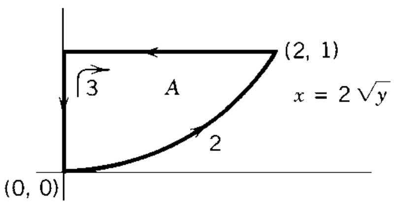
The closed curve C bounding the region A: out from the origin along x=2y to (2,1), back along the horizontal segment, and down the y-axis to the origin.
Figure 6.17. The closed curve \(C\) bounding the region \(A\): out from the origin along \(x=2\sqrt{y}\) to \((2,1)\), back along the horizontal segment, and down the \(y\)-axis to the origin.

Compute the work \(W=\displaystyle\oint_C \vec{F}\cdot d\vec{r}\).

Using Green’s theorem. Since

\begin{equation} \frac{\partial Q}{\partial x}=0,\qquad \frac{\partial P}{\partial y}=x, \end{equation}

we have

\begin{equation} W=\iint_A\!\left(\frac{\partial Q}{\partial x}-\frac{\partial P}{\partial y}\right)dx\,dy =\iint_A (-x)\,dx\,dy =-\int_{y=0}^{1}\!\!\int_{x=0}^{2\sqrt{y}}x\,dx\,dy =-1. \end{equation}

Method Two: Direct Evaluation

\begin{equation} \vec{F}\cdot d\vec{r}=P\,dx+Q\,dy=xy\,dx-y^{2}\,dy. \end{equation}

The boundary is traversed counterclockwise as:

\begin{equation} \begin{aligned} C_1&:\ x=2\sqrt{y},\ (0,0)\to(2,1),\\ C_2&:\ y=1,\ (2,1)\to(0,1),\\ C_3&:\ x=0,\ (0,1)\to(0,0). \end{aligned} \end{equation}

Path \(C_1\): The curve is \(x = 2\sqrt{y}\), or equivalently \(y = \dfrac{x^{2}}{4}\), with \(x:0\to2.\)

\begin{equation} d\vec{r} = \hat{i}\,dx + \hat{j}\,dy, \qquad dy = \frac{x}{2}\,dx. \end{equation}

Then

\begin{equation} \begin{aligned} W_1 &= \int_{0}^{2} \big(xy\,dx - y^{2}\,dy\big) = \int_{0}^{2} \left[x\!\left(\frac{x^{2}}{4}\right) - \left(\frac{x^{2}}{4}\right)^{2}\!\left(\frac{x}{2}\right)\right] dx \\[6pt] &= \int_{0}^{2} \left(\frac{x^{3}}{4} - \frac{x^{5}}{32}\right) dx = \left[\frac{x^{4}}{16} - \frac{x^{6}}{192}\right]_{0}^{2} \\[6pt] &= \left(\frac{16}{16} - \frac{64}{192}\right) = 1 - \frac{1}{3} = \boxed{\frac{2}{3}}. \end{aligned} \end{equation}

Path \(C_2\): \(y=1,\ dy=0,\ x:2\to0\).

\begin{equation} d\vec{r} = \hat{i}\,dx, \qquad \vec{F} = (x, -1). \end{equation}

Thus

\begin{equation} \begin{aligned} W_2 &=\int_{2}^{0} (xy\,dx - y^{2}\,dy) = \int_{2}^{0} x(1)\,dx = \left[\frac{x^{2}}{2}\right]_{2}^{0} =\boxed{-2}. \end{aligned} \end{equation}

Path \(C_3\): \(x=0,\ dx=0,\ y:1\to0\).

\begin{equation} d\vec{r} = \hat{j}\,dy, \qquad \vec{F} = (0, -y^{2}). \end{equation}

Then

\begin{equation} \begin{aligned} W_3 &=\int_{1}^{0} (xy\,dx - y^{2}\,dy) =\int_{1}^{0} (-y^{2})\,dy =\left[-\frac{y^{3}}{3}\right]_{1}^{0} =\boxed{\frac{1}{3}}. \end{aligned} \end{equation}

Total Work (Counterclockwise):

\begin{equation} W = W_1 + W_2 + W_3 = \frac{2}{3} - 2 + \frac{1}{3} = \boxed{-1}. \end{equation}

6.8The Divergence and Stokes’s Theorems

6.8.1The Divergence Theorem in the Plane

Let

\begin{equation} \vec{F}(x,y) = F_x\,\hat{i} + F_y\,\hat{j} \end{equation}

be a continuously differentiable vector field defined on a region \(A\) of the \(xy\)-plane, bounded by a positively oriented (counterclockwise) closed curve \(\partial A\).

To connect this with Green’s theorem, define

\begin{equation} P = -F_y, \qquad Q = F_x. \end{equation}

Then the combination appearing in Green’s theorem,

\begin{equation} \frac{\partial Q}{\partial x} - \frac{\partial P}{\partial y}, \end{equation}

becomes

\begin{equation} \frac{\partial F_x}{\partial x} + \frac{\partial F_y}{\partial y} = \vec{\nabla}\cdot \vec{F}. \end{equation}

Geometric Relation to the Line Integral

Along the curve \(\partial A\), the differential displacement vector is

\begin{equation} d\vec{r} = \hat{i}\,dx + \hat{j}\,dy, \end{equation}

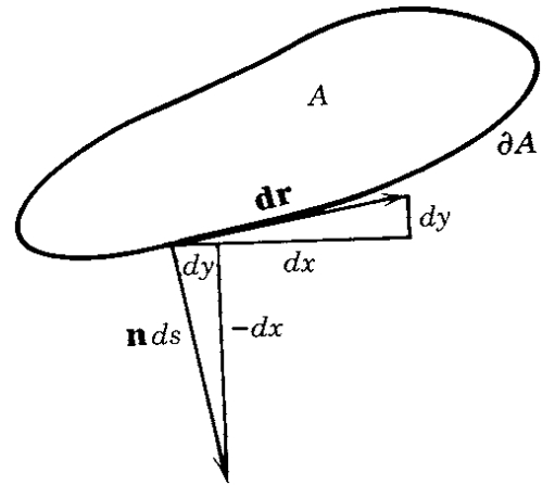
which is tangent to the boundary. The outward normal vector (perpendicular to the tangent) is

\begin{equation} \hat{n}\,ds = \hat{i}\,dy - \hat{j}\,dx, \end{equation}

where \(ds = \sqrt{(dx)^2 + (dy)^2}\) is the differential arc length.

The outward normal on the boundary A: turning dr through a quarter turn gives n\,ds=i\,dy-j\,dx.
Figure 6.18. The outward normal on the boundary \(\partial A\): turning \(d\vec{r}\) through a quarter turn gives \(\hat{n}\,ds=\hat{i}\,dy-\hat{j}\,dx\).

Now, using \(P=-F_y\) and \(Q=F_x\),

\begin{equation} P\,dx + Q\,dy = (-F_y)\,dx + F_x\,dy = (F_x\,\hat{i} + F_y\,\hat{j}) \cdot (\hat{i}\,dy - \hat{j}\,dx) = \vec{F} \cdot \hat{n}\,ds. \end{equation}

Substituting into Green’s theorem gives

\begin{equation} \oint_{\partial A} \vec{F}\cdot\hat{n}\,ds = \iint_A (\vec{\nabla}\cdot\vec{F})\,dx\,dy. \end{equation}
Theorem - Divergence Theorem in Two Dimensions
\begin{equation} \boxed{ \int_A (\vec{\nabla}\cdot\vec{F})\,dA = \oint_{\partial A} \vec{F}\cdot\hat{n}\,ds. } \end{equation}

This states that the total flux of \(\vec{F}\) through the boundary \(\partial A\) equals the integral of the divergence of \(\vec{F}\) over the enclosed region \(A\).

Extension to Three Dimensions (Gauss’s Theorem)

Theorem - Divergence Theorem in Three Dimensions

If \(\vec{F}(x,y,z)\) has continuous partial derivatives within a closed volume \(\tau\) bounded by a closed surface \(\sigma\), then

\begin{equation} \boxed{ \int_{\tau} (\vec{\nabla}\cdot\vec{F})\,d\tau = \oint_{\partial \tau} \vec{F}\cdot d\vec{\sigma}. } \end{equation}
Remark
  • The left-hand side measures the total source strength (divergence) of \(\vec{F}\) within the volume \(V\).

  • The right-hand side measures the total flux of \(\vec{F}\) through the enclosing surface \(S\).

  • Gauss’s theorem thus connects the local divergence of a field to its global outflow.

Example - Field and region

Let

\begin{equation} \vec{F}=\alpha\,z\,\hat{k}, \end{equation}

and let \(\tau\) be the solid right circular cylinder of radius \(R\) and height \(h\) whose axis is the \(z\)-axis, with bottom at \(z=0\) and top at \(z=h\). Its boundary \(\partial\tau=\sigma\) consists of three pieces:

\begin{equation} \sigma = S_1\cup S_2\cup S_3, \quad \begin{cases} S_1:\ \text{bottom disk }(z=0),\\ S_2:\ \text{top disk }(z=h),\\ S_3:\ \text{lateral surface }(\rho=R). \end{cases} \end{equation}

Goal. Verify the Divergence Theorem

\begin{equation} \int_{\tau} (\vec{\nabla}\cdot\vec{F})\,d\tau = \oint_{\partial \tau} \vec{F}\cdot d\vec{\sigma} \end{equation}

for this \(\vec{F}\) and \(\tau\).

  1. Compute the divergence.

    \begin{equation} \vec{\nabla}\cdot\vec{F} =\frac{\partial F_x}{\partial x}+\frac{\partial F_y}{\partial y}+\frac{\partial F_z}{\partial z} =\frac{\partial (\alpha z)}{\partial z}=\alpha. \end{equation}
  2. Evaluate the volume integral. Since \(\vec{\nabla}\cdot\vec{F}=\alpha\) is constant,

    \begin{equation} \int_{\tau} (\vec{\nabla}\cdot\vec{F})\,d\tau =\alpha\int_{\tau} d\tau =\alpha\;(\text{Vol of cylinder}) =\alpha\,\pi R^2 h. \end{equation}
  3. Decompose the surface flux.

    \begin{equation} \oint_{\partial \tau} \vec{F}\cdot d\vec{\sigma} =\iint_{S_1}\vec{F}\cdot d\vec{\sigma} +\iint_{S_2}\vec{F}\cdot d\vec{\sigma} +\iint_{S_3}\vec{F}\cdot d\vec{\sigma}. \end{equation}
  4. Flux through the bottom disk \(S_1\) (at \(z=0\)). The outward normal is \(-\hat{k}\), and on \(S_1\) we have \(\vec{F}=\alpha(0)\hat{k}=\vec{0}\). Hence

    \begin{equation} \iint_{S_1}\vec{F}\cdot d\vec{\sigma}=0. \end{equation}
  5. Flux through the lateral surface \(S_3\) (\(\rho=R\)). Here \(d\vec{\sigma}=\hat{\rho}\,R\,d\phi\,dz\) (outward), while \(\vec{F}=\alpha z\,\hat{k}\) is parallel to \(\hat{k}\). Since \(\hat{k}\cdot\hat{\rho}=0\),

    \begin{equation} \iint_{S_3}\vec{F}\cdot d\vec{\sigma}=0. \end{equation}
  6. Flux through the top disk \(S_2\) (at \(z=h\)). The outward normal is \(+\hat{k}\) and \(\vec{F}=\alpha h\,\hat{k}\) on \(S_2\). Thus

    \begin{equation} \iint_{S_2}\vec{F}\cdot d\vec{\sigma} =\alpha h\iint_{S_2} d\sigma =\alpha h\,(\pi R^2). \end{equation}
  7. Add the contributions.

    \begin{equation} \oint_{\partial \tau} \vec{F}\cdot d\vec{\sigma} = 0 + \alpha h\,\pi R^2 + 0 = \alpha\,\pi R^2 h. \end{equation}
  8. Conclusion (Theorem verified).

    \begin{equation} \boxed{ \int_{\tau} (\vec{\nabla}\cdot\vec{F})\,d\tau = \alpha\,\pi R^2 h = \oint_{\partial \tau} \vec{F}\cdot d\vec{\sigma}. } \end{equation}

    Hence, the Divergence Theorem holds for \(\vec{F}=\alpha z\,\hat{k}\) on the cylindrical region \(\tau\).

Example

Compute

\begin{equation} \oint_{S} \vec{F}\cdot\hat{n}\,d\sigma, \qquad \text{where} \qquad \vec{F}(x,y,z) = x\cos^{2}y\,\hat{i} + xz\,\hat{j} + z\sin^{2}y\,\hat{k}, \end{equation}

and \(S\) is the sphere

\begin{equation} x^{2}+y^{2}+z^{2}=R^{2}, \end{equation}

centered at the origin with radius \(R=3\), and \(\hat{n}\) is the outward unit normal vector.

Solution.

By Gauss’s theorem,

\begin{equation} \oint_{\partial \tau} \vec{F}\cdot d\vec{\sigma} = \iiint_{\tau} (\vec{\nabla}\cdot\vec{F})\,d\tau, \end{equation}

where \(\tau\) is the solid ball enclosed by the surface \(S\).

Thus, the flux through \(S\) equals the triple integral of the divergence of \(\vec{F}\) over the volume of the sphere.

Step 2. Compute the Divergence of \(\vec{F}\).

\begin{equation} \begin{aligned} \vec{\nabla}\cdot\vec{F} &= \frac{\partial F_x}{\partial x} + \frac{\partial F_y}{\partial y} + \frac{\partial F_z}{\partial z} \\[4pt] &= \frac{\partial}{\partial x}\!\left(x\cos^{2}y\right) + \frac{\partial}{\partial y}\!\left(xz\right) + \frac{\partial}{\partial z}\!\left(z\sin^{2}y\right). \end{aligned} \end{equation}

Compute each derivative separately:

\begin{equation} \frac{\partial F_x}{\partial x} = \cos^{2}y, \qquad \frac{\partial F_y}{\partial y} = 0, \qquad \frac{\partial F_z}{\partial z} = \sin^{2}y. \end{equation}

Hence,

\begin{equation} \vec{\nabla}\cdot\vec{F} = \cos^{2}y + 0 + \sin^{2}y = 1. \end{equation}

Step 3. Evaluate the Volume Integral.

Since \(\vec{\nabla}\cdot\vec{F}=1\) everywhere,

\begin{equation} \iiint_{\tau} (\vec{\nabla}\cdot\vec{F})\,d\tau = \iiint_{\tau} 1\,d\tau = \text{Volume of the sphere of radius } R=3. \end{equation}

The volume of a sphere is

\begin{equation} V = \frac{4}{3}\pi R^{3}, \end{equation}

so

\begin{equation} \iiint_{\tau} 1\,d\tau = \frac{4}{3}\pi (3)^{3} = 36\pi. \end{equation}

Step 4. Write the Final Answer.

\begin{equation} \boxed{ \iint_{S} \vec{F}\cdot\hat{n}\,d\sigma = \iiint_{\tau} (\vec{\nabla}\cdot\vec{F})\,d\tau = 36\pi. } \end{equation}
  • Because \(\vec{\nabla}\cdot\vec{F}=1\) everywhere, the flux through any closed surface equals the enclosed volume.

  • In this problem, the direction of \(\hat{n}\) is outward, consistent with Gauss’s theorem.

  • This example illustrates how the divergence theorem transforms a difficult surface integral into a simple volume integral.

6.8.4Stokes’s Theorem in the Plane

Let

\begin{equation} \vec{F}(x,y) = F_x\,\hat{i} + F_y\,\hat{j}, \qquad P = F_x, \quad Q = F_y. \end{equation}

Then the combination in Green’s theorem,

\begin{equation} \frac{\partial Q}{\partial x} - \frac{\partial P}{\partial y} = \frac{\partial F_y}{\partial x} - \frac{\partial F_x}{\partial y} = (\vec{\nabla}\times\vec{F})\cdot\hat{k}, \end{equation}

is the \(z\)-component of the curl of \(\vec{F}\), which represents the local rotation or vorticity.

Using

\begin{equation} d\vec{r} = \hat{i}\,dx + \hat{j}\,dy, \end{equation}

we can write

\begin{equation} P\,dx + Q\,dy = (F_x\,\hat{i} + F_y\,\hat{j}) \cdot (\hat{i}\,dx + \hat{j}\,dy) = \vec{F}\cdot d\vec{r}. \end{equation}

Substituting this into Green’s theorem gives
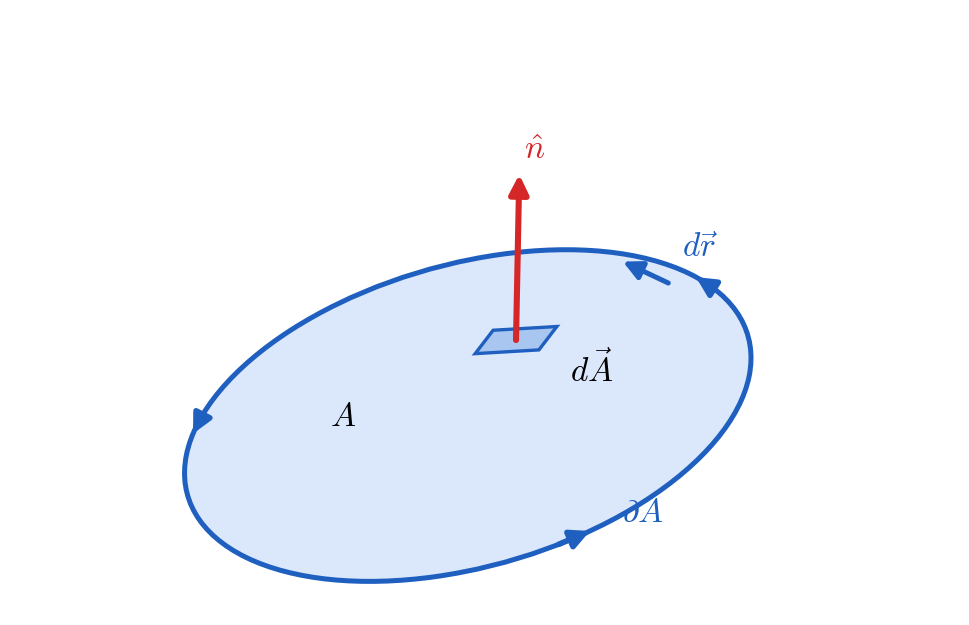
\begin{equation} \int_A (\vec{\nabla}\times\vec{F})\cdot\hat{k}\,dA = \oint_{\partial A} \vec{F}\cdot d\vec{r}. \end{equation}
Theorem - Stokes’s Theorem in Two Dimensions
\begin{equation} \boxed{ \int_A (\vec{\nabla}\times\vec{F})\cdot\hat{k}\,dA = \oint_{\partial A} \vec{F}\cdot d\vec{r}. } \end{equation}
Stokes's theorem: the circulation of F around the boundary equals the flux of F through any surface spanning it.
Figure 6.19. Stokes's theorem: the circulation of \(\vec{F}\) around the boundary equals the flux of \(\vec{\nabla}\times\vec{F}\) through any surface spanning it.

This expresses that the circulation of \(\vec{F}\) around a closed boundary equals the total curl flux through the enclosed region.

Extension to Three Dimensions (General Stokes’s Theorem)

Theorem - Stokes’s Theorem in Three Dimensions

If \(\vec{F}\) has continuous partial derivatives on a smooth surface \(\sigma\) bounded by a positively oriented closed curve \(C\), then

\begin{equation} \boxed{ \int_{\sigma} (\vec{\nabla}\times\vec{F})\cdot d\vec{\sigma}=\oint_{\partial \sigma} \vec{F}\cdot d\vec{r}. } \end{equation}
Remark
  • The line integral \(\oint_{\partial \sigma} \vec{F}\cdot d\vec{r}\) measures the circulation of \(\vec{F}\) along the boundary \(\partial \sigma\).

  • The surface integral \( \int_{\sigma} (\vec{\nabla}\times\vec{F})\cdot d\vec{\sigma}\) measures the total curl flux through the surface \(\sigma\).

  • Stokes’s theorem connects the local rotation of a field to its global circulation.
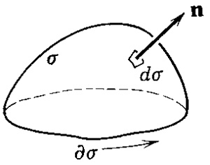
A surface with element d and unit normal n, bounded by the closed curve . The direction of the normal and the sense of the boundary are tied together by the right-hand rule.
Figure 6.20. A surface \(\sigma\) with element \(d\vec{\sigma}\) and unit normal \(\hat{n}\), bounded by the closed curve \(\partial\sigma\). The direction of the normal and the sense of the boundary are tied together by the right-hand rule.
Example - Flux of the Curl over a Hemisphere — Direct Method and Stokes’s Theorem

Let

\begin{equation} \vec{F}(x,y,z) = 4y\,\hat{i} + x\,\hat{j} + 2z\,\hat{k}, \end{equation}

and let \(S\) be the upper hemisphere

\begin{equation} x^{2} + y^{2} + z^{2} = a^{2}, \qquad z \ge 0, \end{equation}

with outward unit normal \(\hat{n}\). We wish to evaluate

\begin{equation} I = \iint_{S} (\vec{\nabla}\times\vec{F}) \cdot \hat{n}\, d\sigma \end{equation}

by two independent methods.

Step 1 — Direct Surface Integral on the Hemisphere.

(a) Compute the curl of \(\vec{F}\).

\begin{equation} \vec{\nabla}\times\vec{F} = \begin{vmatrix} \hat{i} & \hat{j} & \hat{k}\\ \partial_x & \partial_y & \partial_z\\ 4y & x & 2z \end{vmatrix} = \big(0-0\big)\hat{i} -\big(0-0\big)\hat{j} +\big(\partial_x x - \partial_y 4y\big)\hat{k} = (1 - 4)\,\hat{k} = -3\,\hat{k}. \end{equation}

(b) Compute \((\vec{\nabla}\times\vec{F})\cdot\hat{n}\). On the sphere \(r=a\),

\begin{equation} \hat{n} = \frac{\vec{r}}{|\vec{r}|} = \frac{x\,\hat{i} + y\,\hat{j} + z\,\hat{k}}{a}. \end{equation}

Hence

\begin{equation} (\vec{\nabla}\times\vec{F})\cdot\hat{n} = (-3\hat{k})\cdot\frac{\vec{r}}{a} = -\frac{3z}{a}. \end{equation}

(c) Evaluate the surface integral. In spherical coordinates,

\begin{equation} z = a\cos\theta, \qquad d\sigma = a^{2}\sin\theta\,d\theta\,d\phi, \end{equation}

for \(0\le \theta \le \frac{\pi}{2}\), \(0\le \phi \le 2\pi\). Then

\begin{equation} \begin{aligned} I &= \int_{0}^{2\pi}\!\!\int_{0}^{\pi/2} \left(-\frac{3z}{a}\right)a^{2}\sin\theta\,d\theta\,d\phi = -3a^{2}\int_{0}^{2\pi}\!\!d\phi \int_{0}^{\pi/2}\!\!\sin\theta\cos\theta\,d\theta \\[4pt] &= -3a^{2}(2\pi) \left[\frac{1}{2}\sin^{2}\theta\right]_{0}^{\pi/2} = -3a^{2}(2\pi)\!\left(\frac{1}{2}\right) = \boxed{-3\pi a^{2}}. \end{aligned} \end{equation}

Step 2 — Using Stokes’s Theorem (Boundary Method).

By Stokes’s theorem,

\begin{equation} I = \iint_{S} (\vec{\nabla}\times\vec{F})\cdot\hat{n}\,d\sigma = \oint_{C} \vec{F}\cdot d\vec{r}, \end{equation}

where \(C\) is the boundary of the hemisphere:

\begin{equation} C:\ x^{2}+y^{2}=a^{2}, \quad z=0, \end{equation}

oriented counterclockwise as viewed from \(+z\).

(a) Parameterize the boundary.

\begin{equation} \vec{r}(\phi) = a\cos\phi\,\hat{i} + a\sin\phi\,\hat{j}, \qquad d\vec{r} = (-a\sin\phi\,\hat{i} + a\cos\phi\,\hat{j})\,d\phi, \end{equation}

with \(0 \le \phi \le 2\pi.\)

(b) Evaluate \(\vec{F}\) along \(C\). On the circle \(z=0\):

\begin{equation} \vec{F} = 4y\,\hat{i} + x\,\hat{j} = 4a\sin\phi\,\hat{i} + a\cos\phi\,\hat{j}. \end{equation}

(c) Compute \(\vec{F}\cdot d\vec{r}\).

\begin{equation} \begin{aligned} \vec{F}\cdot d\vec{r} &= (4a\sin\phi)(-a\sin\phi) + (a\cos\phi)(a\cos\phi)\,d\phi \\[4pt] &= a^{2}\big(\cos^{2}\phi - 4\sin^{2}\phi\big)\,d\phi. \end{aligned} \end{equation}

(d) Integrate around the circle.

\begin{equation} \begin{aligned} \oint_{C}\vec{F}\cdot d\vec{r} &= a^{2}\int_{0}^{2\pi}(\cos^{2}\phi - 4\sin^{2}\phi)\,d\phi \\[4pt] &= a^{2}\!\left[\int_{0}^{2\pi}\cos^{2}\phi\,d\phi - 4\!\int_{0}^{2\pi}\sin^{2}\phi\,d\phi\right] \\[4pt] &= a^{2}\!\big(\pi - 4\pi\big) = \boxed{-3\pi a^{2}}. \end{aligned} \end{equation}

Result and Interpretation.

\begin{equation} \boxed{ \iint_{S}(\vec{\nabla}\times\vec{F})\cdot\hat{n}\,d\sigma = \oint_{C}\vec{F}\cdot d\vec{r} = -3\pi a^{2}. } \end{equation}
  • Both the direct surface integration and Stokes’s theorem give the same result.

  • The negative sign indicates that the curl \((\vec{\nabla}\times\vec{F})=-3\hat{k}\) points opposite to the outward normal of the upper hemisphere.

  • This example illustrates the power of Stokes’s theorem: the curved surface integral can be replaced by a much simpler line integral around the boundary.

6.9Maxwell’s Equations and the Continuity Equation

1. Differential Form

\begin{equation} \begin{aligned} \vec{\nabla}\cdot\vec{E} &= \frac{\rho}{\varepsilon_0}, && \text{(Gauss’s law for $\vec{E}$)} \\[4pt] \vec{\nabla}\cdot\vec{B} &= 0, && \text{(Gauss’s law for $\vec{B}$)} \\[4pt] \vec{\nabla}\times\vec{E} &= -\,\frac{\partial \vec{B}}{\partial t}, && \text{(Faraday’s law)} \\[4pt] \vec{\nabla}\times\vec{B} &= \mu_0\vec{J} + \mu_0\varepsilon_0\,\frac{\partial \vec{E}}{\partial t}, && \text{(Ampère–Maxwell law)} \end{aligned} \end{equation}

Taking the divergence of the Ampère–Maxwell law and using \(\vec{\nabla}\cdot(\vec{\nabla}\times\vec{B})=0\) gives

\begin{equation} \boxed{ \vec{\nabla}\cdot\vec{J} + \frac{\partial \rho}{\partial t} = 0, } \end{equation}

which is the continuity equation in differential form, expressing local charge conservation.

2. Integral Form via Divergence and Stokes’ Theorems

We now apply the Divergence Theorem

\begin{equation} \boxed{ \oint_{\sigma} \vec{F}\cdot d\vec{\sigma} = \int_{\tau} (\vec{\nabla}\cdot\vec{F})\,d\tau } \end{equation}

and the Stokes’ Theorem

\begin{equation} \boxed{ \oint_{C} \vec{F}\cdot d\vec{r} = \int_{\sigma} (\vec{\nabla}\times\vec{F})\cdot d\vec{\sigma}. } \end{equation}

Applying these to each of Maxwell’s equations:

\begin{equation} \begin{aligned} \text{(i)}\quad &\vec{\nabla}\cdot\vec{E} = \frac{\rho}{\varepsilon_0} &&\Rightarrow& \oint_{\sigma} \vec{E}\cdot d\vec{\sigma} &= \frac{1}{\varepsilon_0}\int_{\tau}\rho\,d\tau = \frac{q_{\text{enc}}}{\varepsilon_0}, && \text{(Gauss’s law for $\vec{E}$)} \\[6pt] \text{(ii)}\quad &\vec{\nabla}\cdot\vec{B} = 0 &&\Rightarrow& \oint_{\sigma} \vec{B}\cdot d\vec{\sigma} &= 0, && \text{(Gauss’s law for $\vec{B}$)} \\[6pt] \text{(iii)}\quad &\vec{\nabla}\times\vec{E} = -\,\frac{\partial \vec{B}}{\partial t} &&\Rightarrow& \oint_{C} \vec{E}\cdot d\vec{r} &= -\,\frac{d}{d t}\int_{\sigma}\vec{B}\cdot d\vec{\sigma}, && \text{(Faraday’s law)} \\[6pt] \text{(iv)}\quad &\vec{\nabla}\times\vec{B} = \mu_0\vec{J} + \mu_0\varepsilon_0\,\frac{\partial \vec{E}}{\partial t} &&\Rightarrow& \oint_{C} \vec{B}\cdot d\vec{r} &= \mu_0\int_{\sigma}\vec{J}\cdot d\vec{\sigma} + \mu_0\varepsilon_0\,\frac{d}{d t}\int_{\sigma}\vec{E}\cdot d\vec{\sigma} \\[3pt] &&&&&= \mu_0 I_{\text{enc}} + \mu_0\varepsilon_0\,\frac{d}{d t}\int_{\sigma}\vec{E}\cdot d\vec{\sigma}, && \text{(Ampère–Maxwell law)} \end{aligned} \end{equation}

3. Continuity Equation in Integral Form

Starting from the differential form

\begin{equation} \vec{\nabla}\cdot\vec{J} + \frac{\partial \rho}{\partial t} = 0, \end{equation}

integrate over a fixed volume \(\tau\):

\begin{equation} \int_{\tau} \left(\vec{\nabla}\cdot\vec{J} + \frac{\partial \rho}{\partial t}\right)d\tau = 0. \end{equation}

Apply the Divergence Theorem to the first term:

\begin{equation} \oint_{\sigma} \vec{J}\cdot d\vec{\sigma} + \frac{d}{d t}\int_{\tau} \rho\,d\tau = 0. \end{equation}

Define

\begin{equation} I_{\text{enc}} = \oint_{\sigma} \vec{J}\cdot d\vec{\sigma}, \qquad q_{\text{enc}} = \int_{\tau} \rho\,d\tau, \end{equation}

so that

\begin{equation} \boxed{ I_{\text{enc}} = -\,\frac{d q_{\text{enc}}}{d t}. } \end{equation}

This expresses charge conservation: the rate of decrease of enclosed charge within the volume \(\tau\) equals the net outward current through its bounding closed surface \(\sigma\).

4. Physical Interpretation

Summary of Key Vector Identities

Theorem - Comprehensive Vector Differential Identities (Cartesian Coordinates)

Let \(\phi\) and \(\psi\) be scalar fields, and \(\vec{A}\), \(\vec{U}\), \(\vec{V}\) be vector fields.

\begin{equation} \begin{aligned} &1.\quad \vec{\nabla}\!\cdot(\vec{\nabla}\phi) = \nabla^{2}\phi, \\[4pt] &2.\quad \vec{\nabla}\!\times(\vec{\nabla}\phi) = \vec{0}, \\[4pt] &3.\quad \vec{\nabla}(\vec{\nabla}\!\cdot\!\vec{V}) = \text{grad div }\vec{V}, \\[4pt] &4.\quad \vec{\nabla}\!\cdot(\vec{\nabla}\!\times\!\vec{V}) = 0, \\[4pt] &5.\quad \vec{\nabla}\!\times(\vec{\nabla}\!\times\!\vec{V}) = \vec{\nabla}(\vec{\nabla}\!\cdot\!\vec{V}) - \nabla^{2}\vec{V}, \\[4pt] &6.\quad \vec{\nabla}(\phi\psi) = \phi\,\vec{\nabla}\psi + \psi\,\vec{\nabla}\phi, \\[4pt] &7.\quad \vec{\nabla}\!\cdot(\phi\vec{V}) = \phi\,(\vec{\nabla}\!\cdot\!\vec{V}) + (\vec{\nabla}\phi)\!\cdot\!\vec{V}, \\[4pt] &8.\quad \vec{\nabla}\!\times(\phi\vec{V}) = \phi\,(\vec{\nabla}\!\times\!\vec{V}) + (\vec{\nabla}\phi)\!\times\!\vec{V}, \\[4pt] &9.\quad \vec{\nabla}(\vec{U}\!\cdot\!\vec{V}) = (\vec{U}\!\cdot\!\vec{\nabla})\vec{V} + (\vec{V}\!\cdot\!\vec{\nabla})\vec{U} + \vec{U}\!\times(\vec{\nabla}\!\times\!\vec{V}) + \vec{V}\!\times(\vec{\nabla}\!\times\!\vec{U}), \\[4pt] &10.\quad \vec{\nabla}\!\times(\vec{U}\!\times\!\vec{V}) = (\vec{V}\!\cdot\!\vec{\nabla})\vec{U} - (\vec{U}\!\cdot\!\vec{\nabla})\vec{V} + \vec{U}\,(\vec{\nabla}\!\cdot\!\vec{V}) - \vec{V}\,(\vec{\nabla}\!\cdot\!\vec{U}), \\[4pt] &11.\quad \nabla^{2}(\phi\psi) = \phi\,\nabla^{2}\psi + \psi\,\nabla^{2}\phi + 2\,(\vec{\nabla}\phi)\!\cdot\!(\vec{\nabla}\psi), \\[4pt] &12.\quad \vec{\nabla}\!\cdot\!(\vec{\nabla}\phi\times\vec{\nabla}\psi) = 0. \end{aligned} \end{equation}
Remark

These relations are essential in fluid dynamics, electromagnetism, and quantum mechanics. They enable transformations of differential equations, simplification of vector expressions, and conversions between integral and differential forms of physical laws.

6.11Where Vector Analysis Is Used

Maxwell's equations, treated twice in this chapter, are the clearest demonstration of what vector analysis is for: four statements about \(\vec{\nabla}\cdot\) and \(\vec{\nabla}\times\) contain the whole of classical electromagnetism, including the existence of light. The same operators do similar work elsewhere.

Remark

One idea unifies the integral theorems of this chapter. Green's theorem, the divergence theorem and Stokes's theorem all say the same thing: the accumulated derivative over a region equals the values on its boundary. In one dimension this is the Fundamental Theorem of Calculus, \(\int_a^b f'\,dt = f(b)-f(a)\). Each theorem here is that statement in a higher dimension, with the derivative replaced by a divergence or a curl, and the endpoints by a closed curve or a closed surface.

For the Interested Reader

Vector analysis is where the geometry and the algebra can easily come apart: it is possible to compute a curl correctly for a whole course without ever picturing what it measures. The first item below is the strongest remedy for that. Everything listed is free.

Seeing divergence and curl

3Blue1Brown builds both operators from what they do to a flowing fluid, and then shows why Maxwell's equations say what they say. Twenty minutes here is worth a great deal of symbol-pushing:

Video

Divergence and curl: the language of Maxwell's equations — 3Blue1Brown
Video thumbnail for Divergence and curl: the language of Maxwell's equations — 3Blue1BrownWatch on YouTube

Open video on YouTube

The operators and the integral theorems

Remark

A note on notation, since it varies more here than in any other chapter. Some books write \(\operatorname{grad}\phi\), \(\operatorname{div}\vec V\) and \(\operatorname{curl}\vec V\) where we write \(\vec{\nabla}\phi\), \(\vec{\nabla}\cdot\vec V\) and \(\vec{\nabla}\times\vec V\); others use \(\operatorname{rot}\vec V\) for the curl. The operator notation used here is worth preferring because it makes identities such as \(\vec{\nabla}\cdot(\vec{\nabla}\times\vec V)=0\) look like what they are — statements about repeated application of one operator.