Chapter 12

Quantum Information and Quantum Computing

12.1Introduction

Earlier chapters asked what a quantum system's energy levels are. This one asks what can be computed with it.

No new postulates. States, operators, the Born rule and the tensor product are the same tools from Chapter 1. One simplification keeps the discussion clear: every Hilbert space here is finite-dimensional. A state is a complex column vector, an observable is a matrix, and each key claim can be verified by hand.

Chapter 1 deferred density operators and entanglement to “advanced courses on quantum information” (Sec. 1.7.4). This chapter is that missing bridge.

Skipped: Shor's algorithm (it needs the quantum Fourier transform), error correcting codes, and open-system theory beyond Sec. 12.13.

The chapter has four objectives: to distinguish a qubit from a classical random bit, to read simple quantum circuits, to establish why interference gives an algorithmic advantage, and to explain why decoherence is the main engineering bottleneck.

Remark 12.1.1A map of the field

Dominic Walliman's Map of Quantum Computing puts the whole field on one page. It serves as a useful companion to this chapter; see Sec. 12.17.

12.2Classical Information

Definition 12.2.1Bit

A bit is a system with two distinguishable states, $0$ and $1$ .

A light switch is the simplest example. It is either up or down, and its state can be determined by inspection. A set of $n$ bits has $2^{n}$ possible configurations.

When the state is not known, as for a flipped coin covered by a hand, it is described by a probability vector:

\begin{matrix} 𝐩 = (\begin{matrix} p_{0} \\ p_{1} \end{matrix}), p_{0}, p_{1} \geq 0, p_{0} + p_{1} = 1 . \end{matrix}

This vector describes incomplete knowledge, not a physical superposition. The coin itself is still either heads or tails.

Operations on one bit, as matrices acting on $𝐩$ :

\begin{matrix} I = (\begin{matrix} 1 & 0 \\ 0 & 1 \end{matrix}), NOT = (\begin{matrix} 0 & 1 \\ 1 & 0 \end{matrix}), M = (\begin{matrix} \frac{1}{2} & \frac{1}{2} \\ \frac{1}{2} & \frac{1}{2} \end{matrix}), \end{matrix}

$M$ means “discard the old bit and replace it with a fair random one”.

Theorem 12.2.1Which matrices act on probability vectors

$M$ maps every probability vector to a probability vector iff every entry is non-negative and every column sums to $1$ — a stochastic matrix.

( $\Rightarrow$ ) $M 𝐞_{j}$ is the $j$ -th column, and $𝐞_{j}$ is a probability vector. ( $\Leftarrow$ ) $M 𝐩 = \sum_{j} p_{j} (M 𝐞_{j})$ is a non-negative combination of probability vectors, totalling $\sum_{j} p_{j} = 1$ .

Reversibility. NOT undoes itself. AND does not: given $a \land b = 0$ , the values of $a$ and $b$ cannot be recovered. AND therefore destroys information. By Landauer's principle, erasing one bit dissipates at least $k_{B} T \ln 2 \approx 3 \times 10^{- 21}$ J at room temperature. In contrast, every ideal quantum gate in this chapter is reversible.

12.3Quantum Information

Definition 12.3.1Qubit

A qubit is a two-dimensional Hilbert space with a chosen orthonormal basis

\begin{matrix} {| 0 ⟩, | 1 ⟩}, ⟨ 0 | 0 ⟩ = ⟨ 1 | 1 ⟩ = 1, ⟨ 0 | 1 ⟩ = 0, \end{matrix}

the computational basis.

Easiest example: a spin- $\frac{1}{2}$ , $| 0 ⟩ = | ↑ ⟩$ , $| 1 ⟩ = | ↓ ⟩$ . Chapter 6's two-level atom does as well. Which system it is matters only in Sec. 12.8.

The chosen basis is part of the definition. A spin has no preferred axis until one is chosen; a qubit is a two-level system together with that computational choice.

\begin{matrix} | ψ ⟩ = α | 0 ⟩ + β | 1 ⟩, α, β \in ℂ, | α |^{2} + | β |^{2} = 1 . \end{matrix}

Compare with Eq. (12.1). Both descriptions use two numbers, but the meaning is different: classical entries are non-negative probabilities, while quantum entries are complex amplitudes whose squared moduli sum to one. Most of the conceptual difference between classical and quantum information comes from this one change.

12.3.1Measurement

Definition 12.3.2Projective measurement

Orthogonal projectors ${{\hat{Π}}_{k}}$ with

\begin{matrix} {\hat{Π}}_{k}^{†} = {\hat{Π}}_{k}, {\hat{Π}}_{j} {\hat{Π}}_{k} = δ_{j k} {\hat{Π}}_{k}, \sum_{k} {\hat{Π}}_{k} = \hat{I}, \end{matrix}

giving outcome $k$ with probability

\begin{matrix} p_{k} = ⟨ ψ | {\hat{Π}}_{k} | ψ ⟩ = {‖ {\hat{Π}}_{k} | ψ ⟩ ‖}^{2}, | ψ_{k} ⟩ = \frac{{\hat{Π}}_{k} | ψ ⟩}{\sqrt{p_{k}}} . \end{matrix}

In the computational basis ${\hat{Π}}_{0} = | 0 ⟩ ⟨ 0 |$ , ${\hat{Π}}_{1} = | 1 ⟩ ⟨ 1 |$ , so $p_{0} = | α |^{2}$ , $p_{1} = | β |^{2}$ .

Two essential differences from classical readout now appear. Measurement changes the state, and one run returns only one classical bit even though the state was described by complex amplitudes.

To measure in another basis ${| u_{k} ⟩}$ , rotate first — hardware typically measures in the computational basis only:

\begin{matrix} | ⟨ u_{k} | ψ ⟩ |^{2} = | ⟨ k | \hat{V} | ψ ⟩ |^{2}, \hat{V} | u_{k} ⟩ = | k ⟩ . \end{matrix}

12.3.2Global Phase

Theorem 12.3.1Global phase is invisible

$| ψ^{'} ⟩ = e^{i γ} | ψ ⟩$ gives identical probabilities, expectation values and evolution.

$| ⟨ k | ψ^{'} ⟩ |^{2} = | e^{i γ} |^{2} | ⟨ k | ψ ⟩ |^{2} = | ⟨ k | ψ ⟩ |^{2}$ ; and $⟨ ψ^{'} | \hat{A} | ψ^{'} ⟩ = e^{- i γ} e^{i γ} ⟨ ψ | \hat{A} | ψ ⟩$ . Linearity carries $e^{i γ}$ through any $\hat{U}$ , so both apply at all later times.

A relative phase is physical: $| 0 ⟩ + | 1 ⟩$ and $| 0 ⟩ - | 1 ⟩$ are orthogonal and therefore experimentally distinguishable. Keeping global and relative phase separate prevents many later mistakes.

12.4What Makes Quantum Information Useful

The central mechanism is interference. Probabilities are non-negative, so classical paths only add. Complex amplitudes can add or cancel, and that controlled cancellation is what quantum algorithms exploit.

Example 12.4.1Randomizing twice

Apply $M$ of Eq. (12.2), and the Hadamard gate $\hat{H} = \frac{1}{\sqrt{2}} (\begin{matrix} 1 & 1 \\ 1 & - 1 \end{matrix})$ , twice each. After one application, both turn a definite input into fifty-fifty outcomes.

Solution.

Classically $M^{2} = M$ : randomizing a random bit leaves it random. Both routes from “ $0$ ” to “ $1$ ” contribute $+ \frac{1}{4}$ , and $\frac{1}{4} + \frac{1}{4}$ cannot vanish.

Quantum mechanically $\hat{H} | 0 ⟩ = | + ⟩$ , also fifty-fifty. But the second Hadamard recombines paths with phase:

\hat{H} | + ⟩ = \frac{| + ⟩ + | - ⟩}{\sqrt{2}} = \frac{1}{2} (| 0 ⟩ + | 1 ⟩ + | 0 ⟩ - | 1 ⟩) = | 0 ⟩ .

The two routes to $| 1 ⟩$ carried $+ \frac{1}{2}$ and $- \frac{1}{2}$ and canceled. As matrices, ${\hat{H}}^{2} = \hat{I}$ while $M$ has no inverse.

	Probabilistic bit	Qubit
State	$𝐩$ , entries $\geq 0$	$\| ψ ⟩$ , entries in $ℂ$
Constraint	$\sum_{j} p_{j} = 1$	$\sum_{j} \| α_{j} \|^{2} = 1$
Operations	stochastic	unitary
Reversible?	only permutations	always
Cancellation?	impossible	routine
Reading it	free, repeatable	disturbs; one bit out
Copying it	free	impossible (Thm. 12.12.1)

Remark 12.4.1

2^{n}

amplitudes is not

2^{n}

answers

An $n$ -qubit state holds $2^{n}$ amplitudes, but measuring returns $n$ bits, corresponding to one random branch. The amplitudes are not an answer sheet; they are a medium in which interference can be engineered. Designing that interference, not “reading all branches,” is the heart of quantum algorithm design.

12.5Qubits and Gates

12.5.1The Bloch Sphere

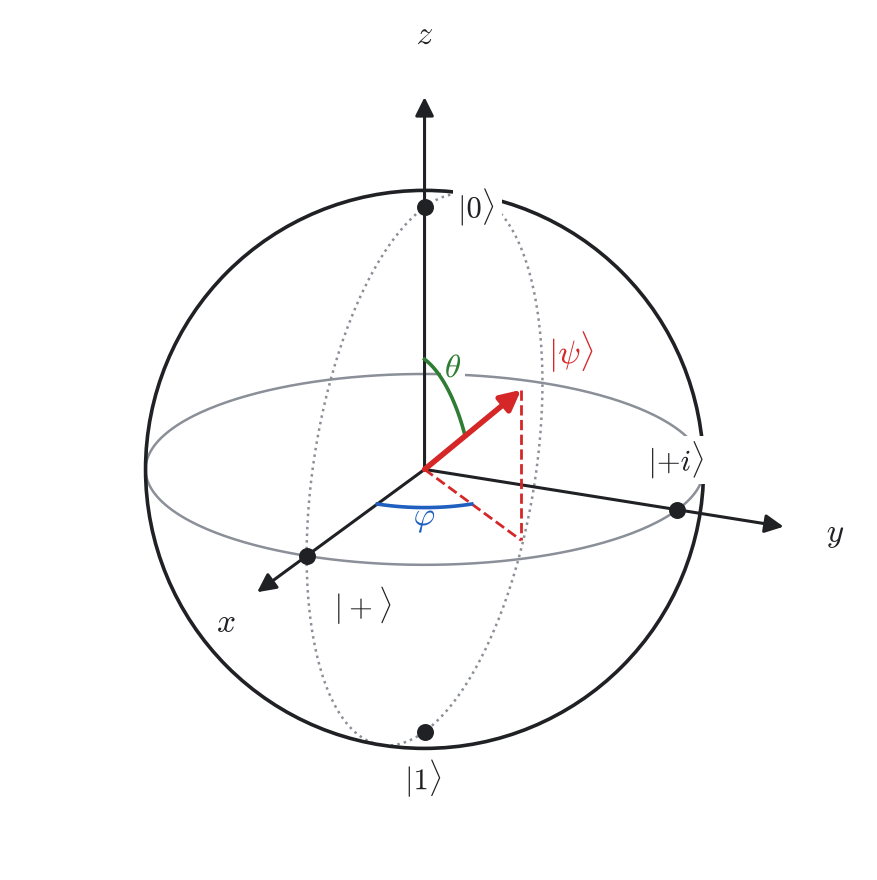
The Bloch sphere is the standard geometric picture for pure one-qubit states. Start from Eq. (12.4) and separate magnitude and phase:

Write $α = r_{0} e^{i γ_{0}}$ , $β = r_{1} e^{i γ_{1}}$ . Divide out $e^{i γ_{0}}$ (Theorem 12.3.1); only $φ = γ_{1} - γ_{0}$ survives. Then $r_{0}^{2} + r_{1}^{2} = 1$ is solved by $r_{0} = \cos (θ / 2)$ , $r_{1} = \sin (θ / 2)$ — which is where the half-angle comes from:

\begin{matrix} | ψ ⟩ = \cos \frac{θ}{2} | 0 ⟩ + e^{i φ} \sin \frac{θ}{2} | 1 ⟩, θ \in [0, π], φ \in [0, 2 π) \end{matrix}

Definition 12.5.1Bloch vector

\begin{matrix} \vec{r} = (⟨ \hat{X} ⟩, ⟨ \hat{Y} ⟩, ⟨ \hat{Z} ⟩), \end{matrix}

with $\hat{X}, \hat{Y}, \hat{Z}$ the Pauli matrices of Eq. (3.26).

Using $⟨ \hat{Z} ⟩ = | α |^{2} - | β |^{2}$ , $⟨ \hat{X} ⟩ = 2 Re (α^{*} β)$ , $⟨ \hat{Y} ⟩ = 2 Im (α^{*} β)$ ,

\begin{matrix} \vec{r} = (\sin θ \cos φ, \sin θ \sin φ, \cos θ), \end{matrix}

the unit vector at $(θ, φ)$ . Pure states lie on the surface; Sec. 12.13 treats mixed states inside the sphere.

The state (/2)0+e^i(/2)1 on the Bloch sphere. States orthogonal in Hilbert space are antipodal here, not perpendicular — the half-angle does that. — Figure 12.1. The state $\cos (θ / 2) | 0 ⟩ + e^{i φ} \sin (θ / 2) | 1 ⟩$ on the Bloch sphere. States *orthogonal* in Hilbert space are *antipodal* here, not perpendicular — the half-angle does that.

Name	State	$(θ, φ)$	$\vec{r}$
$\| 0 ⟩$	$\| 0 ⟩$	$(0, -)$	$+ {\vec{e}}_{z}$
$\| 1 ⟩$	$\| 1 ⟩$	$(π, -)$	$- {\vec{e}}_{z}$
$\| + ⟩$	$\frac{1}{\sqrt{2}} (\| 0 ⟩ + \| 1 ⟩)$	$(π / 2, 0)$	$+ {\vec{e}}_{x}$
$\| - ⟩$	$\frac{1}{\sqrt{2}} (\| 0 ⟩ - \| 1 ⟩)$	$(π / 2, π)$	$- {\vec{e}}_{x}$
$\| + i ⟩$	$\frac{1}{\sqrt{2}} (\| 0 ⟩ + i \| 1 ⟩)$	$(π / 2, π / 2)$	$+ {\vec{e}}_{y}$
$\| - i ⟩$	$\frac{1}{\sqrt{2}} (\| 0 ⟩ - i \| 1 ⟩)$	$(π / 2, 3 π / 2)$	$- {\vec{e}}_{y}$

12.5.2What a Gate Is

Definition 12.5.2Quantum gate

A gate on $n$ qubits is a unitary operator on their $2^{n}$ -dimensional space.

Theorem 12.5.1Which matrices act on state vectors

$\hat{U}$ maps normalized states to normalized states — equivalently preserves inner products — iff ${\hat{U}}^{†} \hat{U} = \hat{I}$ .

If ${\hat{U}}^{†} \hat{U} = \hat{I}$ then $⟨ \hat{U} ψ | \hat{U} φ ⟩ = ⟨ ψ | φ ⟩$ . Conversely $⟨ ψ | ({\hat{U}}^{†} \hat{U} - \hat{I}) | φ ⟩ = 0$ for all $| ψ ⟩, | φ ⟩$ forces ${\hat{U}}^{†} \hat{U} = \hat{I}$ ; in finite dimensions this also gives $\hat{U} {\hat{U}}^{†} = \hat{I}$ .

Theorems 12.2.1 and 12.5.1 are the comparison in two lines: stochastic matrices preserve probability, unitaries preserve amplitudes and inner products. Every gate is reversible; the only irreversible step in this chapter is measurement.

12.6Single-Qubit Gates

\begin{matrix} \hat{X} = (\begin{matrix} 0 & 1 \\ 1 & 0 \end{matrix}), \hat{Y} = (\begin{matrix} 0 & - i \\ i & 0 \end{matrix}), \hat{Z} = (\begin{matrix} 1 & 0 \\ 0 & - 1 \end{matrix}), \hat{H} = \frac{1}{\sqrt{2}} (\begin{matrix} 1 & 1 \\ 1 & - 1 \end{matrix}), \end{matrix}

\begin{matrix} \hat{P} (λ) = (\begin{matrix} 1 & 0 \\ 0 & e^{i λ} \end{matrix}), \hat{S} = \hat{P} (π / 2), \hat{T} = \hat{P} (π / 4) . \end{matrix}

$\hat{X}$ is NOT. $\hat{Z}$ flips the sign of $| 1 ⟩$ : invisible in the computational basis, decisive in the $| \pm ⟩$ basis, where $\hat{Z} | + ⟩ = | - ⟩$ . $\hat{H}$ converts between computational and $| \pm ⟩$ bases and creates superpositions. $\hat{T}$ is the non-Clifford gate in this list; Sec. 12.10.1 explains why that single difference is crucial.

Four identities, each one matrix multiplication:

\begin{matrix} \hat{H} \hat{X} \hat{H} = \hat{Z}, \hat{H} \hat{Z} \hat{H} = \hat{X}, {\hat{S}}^{2} = \hat{Z}, {\hat{T}}^{2} = \hat{S} . \end{matrix}

The first two say bit flip and phase flip are one operation seen in two bases.

12.6.1Every Gate Is a Rotation

Definition 12.6.1Rotation operators

\begin{matrix} {\hat{R}}_{\vec{n}} (θ) = \exp (- \frac{i θ}{2} \vec{n} \cdot \vec{σ}), \vec{n} \cdot \vec{σ} = n_{x} \hat{X} + n_{y} \hat{Y} + n_{z} \hat{Z} . \end{matrix}

Theorem 12.6.1Closed form

\begin{matrix} {\hat{R}}_{\vec{n}} (θ) = \cos \frac{θ}{2} \hat{I} - i \sin \frac{θ}{2} \vec{n} \cdot \vec{σ} \end{matrix}

and it rotates the Bloch vector by $θ$ about $\vec{n}$ .

Everything rests on $(\vec{n} \cdot \vec{σ})^{2} = \hat{I}$ . From $σ_{i} σ_{j} = δ_{i j} \hat{I} + i ε_{i j k} σ_{k}$ ,

(\vec{n} \cdot \vec{σ})^{2} = \sum_{i, j} n_{i} n_{j} δ_{i j} \hat{I} + i \sum_{i, j, k} ε_{i j k} n_{i} n_{j} σ_{k} = | \vec{n} |^{2} \hat{I} = \hat{I},

the second sum vanishing because $ε_{i j k}$ is antisymmetric in $i \leftrightarrow j$ and $n_{i} n_{j}$ symmetric. With $\hat{A} = \vec{n} \cdot \vec{σ}$ , so ${\hat{A}}^{2 k} = \hat{I}$ and ${\hat{A}}^{2 k + 1} = \hat{A}$ , split the exponential series into even and odd powers to get $\cos (θ / 2) \hat{I} - i \sin (θ / 2) \hat{A}$ . The geometric statement is Exercise E3.

Theorem 12.6.2Every single-qubit gate is a rotation

Every $2 \times 2$ unitary is $\hat{U} = e^{i γ} {\hat{R}}_{\vec{n}} (θ)$ .

Put $e^{i γ} = (\det \hat{U})^{1 / 2}$ , so $\hat{V} = e^{- i γ} \hat{U}$ has $\det \hat{V} = 1$ and hence the form $(\begin{matrix} u & v \\ - v^{*} & u^{*} \end{matrix})$ with $| u |^{2} + | v |^{2} = 1$ . Setting $u = a_{0} - i a_{3}$ , $v = - a_{2} - i a_{1}$ with real $a_{i}$ , expanding $a_{0} \hat{I} - i (a_{1} \hat{X} + a_{2} \hat{Y} + a_{3} \hat{Z})$ reproduces $\hat{V}$ , and $\sum_{i} a_{i}^{2} = 1$ . So $a_{0} = \cos (θ / 2)$ and $(a_{1}, a_{2}, a_{3}) = \sin (θ / 2) \vec{n}$ , which is Eq. (12.15).

Example 12.6.1Hadamard as a rotation

Find its axis and angle.

Solution.

$\hat{H} = \frac{1}{\sqrt{2}} (\hat{X} + \hat{Z}) = \vec{n} \cdot \vec{σ}$ with $\vec{n} = \frac{1}{\sqrt{2}} (1, 0, 1)$ . At $θ = π$ , Eq. (12.15) gives ${\hat{R}}_{\vec{n}} (π) = - i \vec{n} \cdot \vec{σ} = - i \hat{H}$ , so $\hat{H} = e^{i π / 2} {\hat{R}}_{\vec{n}} (π)$ : a half turn about the axis halfway between $x$ and $z$ . That exchanges the $+ z$ and $+ x$ poles, which is $| 0 ⟩ \leftrightarrow | + ⟩$ ; and ${\hat{H}}^{2} = \hat{I}$ because two half turns make a full one.

12.7Making a Gate: From Pulse to Rotation

This section connects abstract gates to laboratory control. The same driven two-level dynamics from Chapter 6 produces these gates directly, and the rotation angle is set by pulse area.

Take Chapter 6's rotating-wave equations, Eq. (6.15), with $| 0 ⟩$ the ground state ( $c_{1}$ ) and $| 1 ⟩$ the excited state ( $c_{2}$ ). Move to the frame rotating at the drive frequency,

\begin{matrix} c_{1} = e^{- i Δ t / 2} b_{1}, c_{2} = e^{+ i Δ t / 2} b_{2}, \end{matrix}

so the first equation becomes

\begin{matrix} e^{- i Δ t / 2} (i {\dot{b}}_{1} + \frac{Δ}{2} b_{1}) = \frac{Ω}{2} e^{- i Δ t} e^{+ i Δ t / 2} b_{2} = \frac{Ω}{2} e^{- i Δ t / 2} b_{2}, \end{matrix}

and, with the second, after cancelling exponentials

\begin{matrix} i {\dot{b}}_{1} = - \frac{Δ}{2} b_{1} + \frac{Ω}{2} b_{2}, i {\dot{b}}_{2} = \frac{Ω}{2} b_{1} + \frac{Δ}{2} b_{2} . \end{matrix}

The explicit time dependence is gone. Reading off the matrix,

\begin{matrix} {\hat{H}}_{rot} = \frac{ℏ}{2} (\begin{matrix} - Δ & Ω \\ Ω & Δ \end{matrix}) = \frac{ℏ}{2} (Ω \hat{X} - Δ \hat{Z}) \end{matrix}

A drive phase $ϕ$ replaces $Ω \hat{X}$ by $Ω (\cos ϕ \hat{X} + \sin ϕ \hat{Y})$ .

Theorem 12.7.1A driven two-level system executes a rotation

Driving for time $t$ at Rabi frequency $Ω$ , detuning $Δ$ and phase $ϕ$ applies

\begin{matrix} \hat{U} (t) = {\hat{R}}_{\vec{n}} (θ), θ = Ω_{R} t, \vec{n} = \frac{(Ω \cos ϕ, Ω \sin ϕ, - Δ)}{Ω_{R}}, \end{matrix}

with $Ω_{R} = \sqrt{Ω^{2} + Δ^{2}}$ . For a shaped pulse the angle is the pulse area $θ = \int Ω d t$ .

${\hat{H}}_{rot} = \frac{ℏ}{2} Ω_{R} \vec{n} \cdot \vec{σ}$ , so $e^{- i {\hat{H}}_{rot} t / ℏ}$ is Eq. (12.14) with $θ = Ω_{R} t$ .

Three consequences are used constantly in hardware control.

Resonant driving rotates in the equatorial plane. $Δ = 0$ puts $\vec{n}$ in the $x y$ plane and $ϕ$ chooses where. A resonant $π$ pulse with $ϕ = 0$ gives ${\hat{R}}_{{\vec{e}}_{x}} (π) = - i \hat{X}$ — Chapter 6's population inversion, relabelled.

Detuning alone gives a $\hat{Z}$ rotation. $Ω = 0$ gives ${\hat{R}}_{- {\vec{e}}_{z}} (Δ t)$ . No pulse needed, which is why machines implement $\hat{Z}$ by shifting the phase of later pulses: essentially zero duration and usually very low error.

Hadamard is two pulses. With $ϕ = π / 2$ and $θ = π / 2$ ,

\begin{matrix} {\hat{R}}_{{\vec{e}}_{y}} (π / 2) = \frac{1}{\sqrt{2}} (\begin{matrix} 1 & - 1 \\ 1 & 1 \end{matrix}), \hat{X} {\hat{R}}_{{\vec{e}}_{y}} (π / 2) = \hat{H} . \end{matrix}

Excited-state population against pulse area, Eq. (6.16). On resonance the area alone fixes the gate. Off resonance the oscillation never reaches 1, so a detuned pulse cannot be made into an X gate by adjusting its duration. — Figure 12.2. Excited-state population against pulse area, Eq. (6.16). On resonance the area alone fixes the gate. Off resonance the oscillation never reaches $1$ , so a detuned pulse cannot be made into an $\hat{X}$ gate by adjusting its duration.

Remark 12.7.1Consistency check

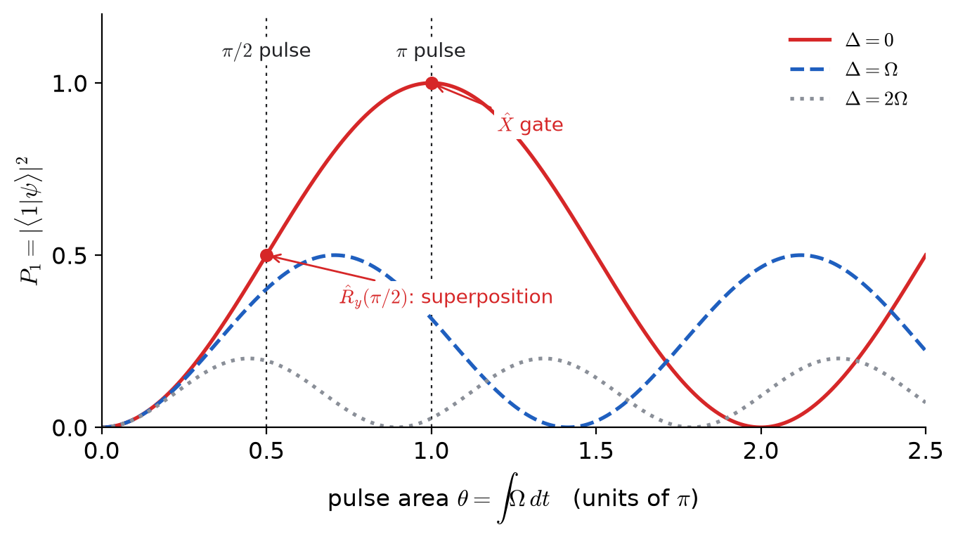
From Eq. (12.15), $⟨ 1 | {\hat{R}}_{\vec{n}} (θ) | 0 ⟩ = - i (Ω / Ω_{R}) \sin (Ω_{R} t / 2)$ , whose modulus squared is Eq. (6.16) exactly. The gate picture and the Rabi picture are one calculation.

Example 12.7.1Calibrating a gate

A superconducting qubit is driven at $Ω / 2 π = 25$ MHz on resonance. (a) How long is an $\hat{X}$ gate? (b) The amplitude drifts high by $1 %$ ; what is the error?

Solution.

(a) $θ = Ω t = π$ gives

t_{π} = \frac{π}{Ω} = \frac{1}{5.0 \times 10^{7} s^{- 1}} = 20 ns .

(b) Area $π (1 + δ)$ instead of $π$ , so

ϵ = 1 - \sin^{2} (\frac{π (1 + δ)}{2}) = \sin^{2} (\frac{π δ}{2}) \approx (\frac{π δ}{2})^{2} = 2.5 \times 10^{- 4}

for $δ = 0.01$ . The error is quadratic in the miscalibration: $1 %$ buys $10^{- 4}$ , and reaching $10^{- 4}$ needs only $δ < 0.64 %$ .

12.8Coherence and Hardware

Real qubits are never perfectly isolated, so two different noise mechanisms must be tracked separately.

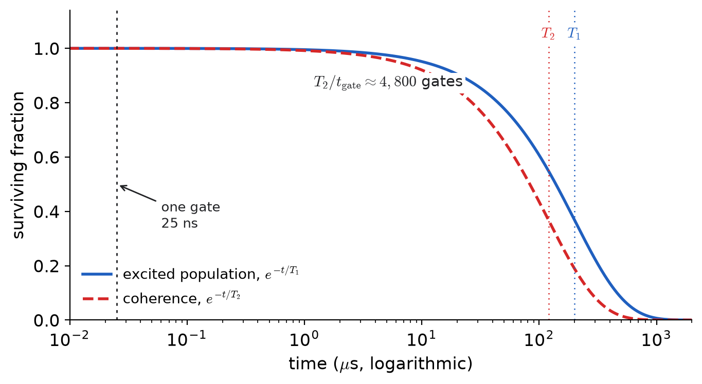
Definition 12.8.1Relaxation and coherence times

$T_{1}$ , the relaxation time: an excited qubit decays, $P_{1} (t) = P_{1} (0) e^{- t / T_{1}}$ . Energy leaves.

$T_{2}$ , the coherence or dephasing time: a superposition loses its relative phase. No energy leaves; the phase becomes unknown.

On the Bloch sphere: $T_{1}$ pulls $\vec{r}$ toward the pole, $T_{2}$ shrinks its equatorial component. So $| + ⟩$ is fragile to dephasing, while $| 0 ⟩$ and $| 1 ⟩$ are unaffected by pure phase noise.

Example 12.8.1Dephasing is not decay

Let the relative phase of $| + ⟩$ drift by an unknown $ϕ$ .

Solution.

The state is $\frac{1}{\sqrt{2}} (| 0 ⟩ + e^{i ϕ} | 1 ⟩)$ . In the computational basis the answer is $\frac{1}{2}$ , $\frac{1}{2}$ for any $ϕ$ : nothing decayed, populations untouched.

In the $| \pm ⟩$ basis, $ϕ = 0$ gives $| + ⟩$ with certainty; averaged over unknown $ϕ$ it is fifty-fifty. What is gone is the interference of Example 12.4.1, on which the whole subject depends, while the populations remain unchanged. This is why $T_{2}$ , not $T_{1}$ , limits computation. Section 12.13 writes it down properly.

\begin{matrix} T_{2} \leq 2 T_{1}, N_{gates} \sim \frac{T_{2}}{t_{gate}} . \end{matrix}

The first because energy decay also destroys phase. The second is the only figure of merit that matters: not lifetime, not speed, but how many operations fit inside the coherence.

The two decays. T1 empties the excited state; T2 destroys the coherence that makes interference possible, at least twice as fast. The dotted line is one gate time for a superconducting qubit. — Figure 12.3. The two decays. $T_{1}$ empties the excited state; $T_{2}$ destroys the coherence that makes interference possible, at least twice as fast. The dotted line is one gate time for a superconducting qubit.

12.8.1What Qubits Are Made Of

Every platform below is a two-level system driven near resonance — that is, every one is Chapter 6, and Theorem 12.7.1 applies unchanged to all of them.

Platform	The two levels	Control	Coherence
Superconducting	lowest two of an	microwave	$10^{2}$ – $10^{3} μ$ s
(transmon)	anharmonic circuit	pulses	gates $\sim 20$ ns
[3pt] Trapped ion	two atomic levels	lasers,	seconds
	of an ion	microwaves	gates $\sim 10 μ$ s
[3pt] Neutral atom	atomic levels;	lasers	seconds
	Rydberg for coupling
[3pt] Photonic	polarization or path	interferometers	loss, not decay
[3pt] Spin	electron or nuclear	microwaves,	ms (NV center)
(dot, donor, NV)	spin- $\frac{1}{2}$	magnetic fields
[3pt] Topological	non-abelian anyons	braiding	in principle immune

Superconducting qubits emphasize fast gates and integration but have shorter coherence. Trapped ions offer much longer coherence but slower gates. When compared through $N_{gates} \sim T_{2} / t_{gate}$ , their effective computational windows are closer than raw coherence times alone suggest. Topological qubits remain the most speculative platform.

12.9Two Qubits

Two qubits already introduce genuinely new behavior because the joint space is $2 \times 2 = 4$ dimensional:

\begin{matrix} | 00 ⟩, | 01 ⟩, | 10 ⟩, | 11 ⟩, | a b ⟩ \equiv | a ⟩ \otimes | b ⟩ . \end{matrix}

As columns and matrices, the tensor product is the Kronecker product:

\begin{matrix} (\begin{matrix} α_{0} \\ α_{1} \end{matrix}) \otimes (\begin{matrix} β_{0} \\ β_{1} \end{matrix}) = (\begin{matrix} α_{0} β_{0} \\ α_{0} β_{1} \\ α_{1} β_{0} \\ α_{1} β_{1} \end{matrix}), (\hat{A} \otimes \hat{B}) (| ψ ⟩ \otimes | φ ⟩) = \hat{A} | ψ ⟩ \otimes \hat{B} | φ ⟩ . \end{matrix}

Remark 12.9.1Qubit ordering

Here the left symbol is the first tensor factor. Qiskit puts qubit $0$ on the right, which swaps the middle two rows and columns of controlled-gate matrices. This is only a convention, but mixing conventions is a common source of errors.

12.9.1Entanglement

Definition 12.9.1Product and entangled

$| Ψ ⟩$ is a product state if $| Ψ ⟩ = | ψ ⟩ \otimes | φ ⟩$ , and entangled otherwise.

Theorem 12.9.1The Bell state is entangled

$| Φ^{+} ⟩ = \frac{1}{\sqrt{2}} (| 00 ⟩ + | 11 ⟩)$ does not factorize.

If $(a | 0 ⟩ + b | 1 ⟩) \otimes (c | 0 ⟩ + d | 1 ⟩)$ , matching coefficients needs $a c = b d = \frac{1}{\sqrt{2}}$ and $a d = b c = 0$ . From $a c \neq 0$ , $a \neq 0$ , so $a d = 0$ forces $d = 0$ — contradicting $b d \neq 0$ .

Definition 12.9.2Bell basis

\begin{matrix} | Φ^{\pm} ⟩ = \frac{| 00 ⟩ \pm | 11 ⟩}{\sqrt{2}}, | Ψ^{\pm} ⟩ = \frac{| 01 ⟩ \pm | 10 ⟩}{\sqrt{2}} . \end{matrix}

An intuitive picture is two perfectly correlated coins. Example 12.9.2 shows that this agreement survives a change of measurement basis.

Remark 12.9.2An entangled state met earlier

Chapter 5's spin singlet is $| Ψ^{-} ⟩$ . Entanglement is what antisymmetrization has been doing since then. One caution: for identical particles some of it is bookkeeping, required by statistics; for distinguishable qubits it is entirely physical.

12.9.2Controlled Gates

Definition 12.9.3Controlled-

\hat{U}

\begin{matrix} {\hat{C}}_{U} = | 0 ⟩ ⟨ 0 | \otimes \hat{I} + | 1 ⟩ ⟨ 1 | \otimes \hat{U} \end{matrix}

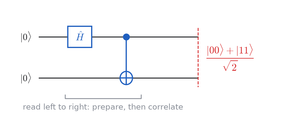
Operationally: if the control is $| 0 ⟩$ , do nothing; if it is $| 1 ⟩$ , apply $\hat{U}$ to the target. If the control is in superposition, linearity applies both branches at once; this is the circuit-level route to entanglement.

With $\hat{U} = \hat{X}$ :

\begin{matrix} CNOT = (\begin{matrix} 1 & 0 & 0 & 0 \\ 0 & 1 & 0 & 0 \\ 0 & 0 & 0 & 1 \\ 0 & 0 & 1 & 0 \end{matrix}), CNOT | a, b ⟩ = | a, a \oplus b ⟩ . \end{matrix}

With $\hat{U} = \hat{Z}$ , $CZ = diag (1, 1, 1, - 1)$ , which is symmetric, so that there is no way to tell which qubit was the control.

Example 12.9.1The simplest entangling circuit

Apply $\hat{H}$ to the first qubit, then $CNOT$ .

Solution.

(\hat{H} \otimes \hat{I}) | 00 ⟩ = \frac{| 00 ⟩ + | 10 ⟩}{\sqrt{2}} \overset{CNOT}{\to} \frac{| 00 ⟩ + | 11 ⟩}{\sqrt{2}} = | Φ^{+} ⟩ .

The other inputs give $| 01 ⟩ \mapsto | Ψ^{+} ⟩$ , $| 10 ⟩ \mapsto | Φ^{-} ⟩$ , $| 11 ⟩ \mapsto | Ψ^{-} ⟩$ . Since an orthonormal basis maps to an orthonormal basis it is unitary. Run backward, it converts the Bell basis to the computational basis, i.e. a Bell measurement, which is the key primitive used throughout Sec. 12.12.

Figure 12.4. The circuit of Example 12.9.1. Read right to left, the circuit performs a Bell measurement.

Example 12.9.2The correlation survives a change of basis

Both parties measure their half of $| Φ^{+} ⟩$ , first in the computational basis, then in the $| \pm ⟩$ basis.

Solution.

Computational: no $| 01 ⟩$ or $| 10 ⟩$ component, so those outcomes have probability zero and the results always agree.

Substituting $| 0 ⟩ = \frac{1}{\sqrt{2}} (| + ⟩ + | - ⟩)$ and $| 1 ⟩ = \frac{1}{\sqrt{2}} (| + ⟩ - | - ⟩)$ , the mixed terms cancel:

| Φ^{+} ⟩ = \frac{| + + ⟩ + | - - ⟩}{\sqrt{2}} .

Same form, so they agree again. Yet each qubit alone is a fair coin in both bases (Eq. (12.49)). No assignment of definite values reproduces this and the intermediate angles too; Sec. 12.12.4 makes that quantitative.

12.10Many Qubits

For $n$ qubits, basis states $| x ⟩$ are labeled by $n$ -bit strings:

\begin{matrix} | Ψ ⟩ = \sum_{x \in {0, 1}^{n}} c_{x} | x ⟩, \sum_{x} | c_{x} |^{2} = 1 . \end{matrix}

$2^{n}$ amplitudes are required; storing $50$ qubits exactly already needs about $16$ petabytes.

Two identities drive the algorithm section that follows:

\begin{matrix} {\hat{H}}^{\otimes n} | 00 \dots 0 ⟩ = \frac{1}{\sqrt{2^{n}}} \sum_{x} | x ⟩, \end{matrix}

an equal superposition of all $2^{n}$ strings from $n$ gates, and

\begin{matrix} {\hat{H}}^{\otimes n} | x ⟩ = \frac{1}{\sqrt{2^{n}}} \sum_{z} (- 1)^{x \cdot z} | z ⟩, x \cdot z = \sum_{i} x_{i} z_{i} mod 2, \end{matrix}

which follows from $\hat{H} | x_{i} ⟩ = \frac{1}{\sqrt{2}} (| 0 ⟩ + (- 1)^{x_{i}} | 1 ⟩)$ on each qubit.

Definition 12.10.1Quantum circuit

A quantum circuit is a sequence of gates on specified qubits (one line per qubit, read left to right). Algebraically, the whole circuit is one unitary:

\begin{matrix} {\hat{U}}_{circuit} = {\hat{U}}_{L} \dots {\hat{U}}_{2} {\hat{U}}_{1}, \end{matrix}

where the order is reversed because state vectors are multiplied from the right.

Example 12.10.1Control is not absolute

Conjugating $CNOT$ by Hadamards on both qubits swaps control and target.

Solution.

Push the Hadamards inside Eq. (12.26), using $\hat{H} | 0 ⟩ = | + ⟩$ , $\hat{H} | 1 ⟩ = | - ⟩$ and $\hat{H} \hat{X} \hat{H} = \hat{Z}$ :

| + ⟩ ⟨ + | \otimes \hat{I} + | - ⟩ ⟨ - | \otimes \hat{Z} = \frac{1}{2} (\hat{I} \otimes \hat{I} + \hat{I} \otimes \hat{Z} + \hat{X} \otimes \hat{I} - \hat{X} \otimes \hat{Z}),

using $| \pm ⟩ ⟨ \pm | = \frac{1}{2} (\hat{I} \pm \hat{X})$ . Expanding a CNOT controlled by the second qubit gives the same operator. Which qubit is “the control” is a statement about the basis, not the physics.

12.10.1Universality

Theorem 12.10.1Universality, without proof

${\hat{H}, \hat{T}, CNOT}$ approximates any $n$ -qubit unitary to any $ε$ ; Solovay–Kitaev needs only $O (\ln^{c} (1 / ε))$ gates per single-qubit gate.

Two caveats and one payoff. First, universality does not imply efficiency: a generic $n$ -qubit unitary still needs about $4^{n}$ elementary gates. Second, $\hat{H}$ together with $CNOT$ is still not universal; this is the Clifford set, which remains efficiently classically simulable (Gottesman–Knill). The non-Clifford gate $\hat{T}$ is what breaks that simulability. The payoff is practical: scalable quantum computing reduces to implementing a small gate set with very high fidelity.

12.11Three Quantum Algorithms

All three algorithms share one structure: prepare superposition, encode information about $f$ into phase, interfere, then measure. The complexity question is the same each time: how many oracle calls are required?

12.11.1The Oracle and Phase Kickback

The map $| x ⟩ \mapsto | f (x) ⟩$ is generally irreversible. To make a unitary oracle, add one target qubit:

\begin{matrix} {\hat{U}}_{f} | x ⟩ | y ⟩ = | x ⟩ | y \oplus f (x) ⟩, \end{matrix}

reversible because $y \oplus f \oplus f = y$ .

Theorem 12.11.1Phase kickback

\begin{matrix} {\hat{U}}_{f} | x ⟩ | - ⟩ = (- 1)^{f (x)} | x ⟩ | - ⟩ \end{matrix}

${\hat{U}}_{f} | x ⟩ \frac{1}{\sqrt{2}} (| 0 ⟩ - | 1 ⟩) = | x ⟩ \frac{1}{\sqrt{2}} (| f (x) ⟩ - | 1 \oplus f (x) ⟩)$ . For $f (x) = 0$ the bracket is $| 0 ⟩ - | 1 ⟩$ ; for $f (x) = 1$ it is $| 1 ⟩ - | 0 ⟩$ . Both equal $(- 1)^{f (x)} \sqrt{2} | - ⟩$ .

The value of $f (x)$ is now stored in a phase factor, where interference can act on it. The auxiliary qubit returns to $| - ⟩$ and can be ignored in later analysis.

12.11.2Deutsch: One Query Instead of Two

Problem. $f : {0, 1} \to {0, 1}$ is constant ( $f (0) = f (1)$ ) or balanced. Which? Classically needs two evaluations.

Circuit. Prepare $| 0 ⟩ | 1 ⟩$ ; $\hat{H}$ on both; ${\hat{U}}_{f}$ ; $\hat{H}$ on the first; measure the first.

Theorem 12.11.2Deutsch

The measurement gives $0$ for constant and $1$ for balanced, with certainty, after one call.

After the Hadamards, $| + ⟩ | - ⟩$ . Kickback on each term gives

\frac{(- 1)^{f (0)} | 0 ⟩ + (- 1)^{f (1)} | 1 ⟩}{\sqrt{2}} | - ⟩ .

Drop the overall $(- 1)^{f (0)}$ (Theorem 12.3.1); the first register is $| + ⟩$ if $f (0) = f (1)$ and $| - ⟩$ otherwise. The final $\hat{H}$ sends these to $| 0 ⟩$ and $| 1 ⟩$ .

Remark 12.11.1What was gained

The algorithm never learns $f (0)$ or $f (1)$ — it learns $f (0) \oplus f (1)$ , a global property, without learning either value. This is the general form of the speed-ups considered here: not many answers at once, but a single question about all of them.

12.11.3Bernstein–Vazirani: $n$ Bits in One Query

Problem. $f (x) = a \cdot x mod 2$ for a hidden $n$ -bit string $a$ . Find $a$ . Classically $n$ queries, one bit at a time.

Circuit. ${| 0 ⟩}^{\otimes n} | 1 ⟩$ ; $\hat{H}$ everywhere; ${\hat{U}}_{f}$ ; ${\hat{H}}^{\otimes n}$ on the first register; measure.

Theorem 12.11.3Bernstein–Vazirani

The measurement returns $a$ with certainty, after one call.

Kickback turns Eq. (12.29) into $2^{- n / 2} \sum_{x} (- 1)^{a \cdot x} | x ⟩$ . Applying Eq. (12.30),

\frac{1}{2^{n}} \sum_{z} [\sum_{x} (- 1)^{x \cdot (a \oplus z)}] | z ⟩ .

The inner sum is $2^{n}$ for $z = a$ and zero otherwise, since for $a \oplus z \neq 0$ the terms cancel in pairs. The state is $| a ⟩$ .

Example 12.11.1

n = 2

a = 11

Solution.

$a \cdot x = x_{1} \oplus x_{2}$ , so the kickback signs are $+, -, -, +$ :

\frac{1}{2} (| 00 ⟩ - | 01 ⟩ - | 10 ⟩ + | 11 ⟩) = | - ⟩ | - ⟩ .

It factorizes, and $\hat{H} | - ⟩ = | 1 ⟩$ on each qubit gives $| 11 ⟩ = | a ⟩$ .

12.11.4Grover: Searching in $\sqrt{N}$

Problem. $f (x) = 1$ for exactly one marked string $w$ among $N = 2^{n}$ . Find $w$ . Classically $N / 2$ calls on average.

Idea. Start from the equal superposition and repeat two steps:

Mark. ${\hat{U}}_{w} = \hat{I} - 2 | w ⟩ ⟨ w |$ flips the sign of the marked amplitude.
Reflect about the average. ${\hat{U}}_{s} = 2 | s ⟩ ⟨ s | - \hat{I}$ sends $c_{x} \mapsto 2 \bar{c} - c_{x}$ .

Step 1 puts the marked amplitude furthest below the average; step 2 lifts it furthest.

Theorem 12.11.4Grover

After $k$ rounds the marked amplitude is $\sin ((2 k + 1) ϑ)$ with $\sin ϑ = 1 / \sqrt{N}$ , so the best choice is

\begin{matrix} k \approx \frac{π}{4 ϑ} - \frac{1}{2} \approx \frac{π}{4} \sqrt{N} . \end{matrix}

The dynamics stays in the two-dimensional plane spanned by $| w ⟩$ and the equal superposition of unmarked states. In that plane, each Grover round is a rotation by $2 ϑ$ toward $| w ⟩$ .

Example 12.11.2Four items, one query, certainty

$N = 4$ , two qubits, marked item $w = 10$ .

Solution.

$\sin ϑ = \frac{1}{2}$ so $ϑ = 30^{\circ}$ , and Theorem 12.11.4 gives $\sin (3 \times 30^{\circ}) = 1$ after one round. Directly: all amplitudes start at $\frac{1}{2}$ ; the oracle flips $| 10 ⟩$ , making the mean $\bar{c} = \frac{1}{4} (\frac{1}{2} + \frac{1}{2} - \frac{1}{2} + \frac{1}{2}) = \frac{1}{4}$ ; reflecting, $c \mapsto 2 \bar{c} - c$ , sends

\frac{1}{2} \mapsto 0, - \frac{1}{2} \mapsto 1 .

The state is exactly $| 10 ⟩$ . Classically one would expect to open two or three of the four boxes.

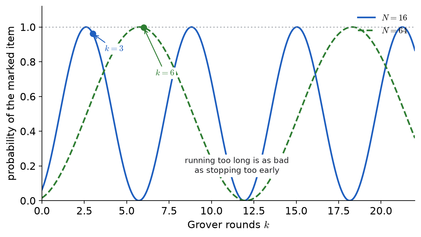
Grover amplification: ^2((2k+1)) rises to near certainty after about 4N rounds, then falls again. Running too long is as bad as stopping too early. — Figure 12.5. Grover amplification: $\sin^{2} ((2 k + 1) ϑ)$ rises to near certainty after about $\frac{π}{4} \sqrt{N}$ rounds, then *falls* again. Running too long is as bad as stopping too early.

Remark 12.11.2A square root is not an exponential

Grover is quadratic and provably optimal for unstructured search: $10^{12}$ entries need $10^{6}$ queries, not $10^{12}$ . Shor's algorithm is the exponential one, and can be because factoring has structure that search lacks.

12.12What Entanglement Is Good For

This section shows what entanglement enables operationally: communication tasks and nonclassical correlations.

12.12.1Three Impossibilities

Theorem 12.12.1No cloning

No unitary $\hat{U}$ and fixed $| s ⟩$ satisfy $\hat{U} (| ψ ⟩ \otimes | s ⟩) = | ψ ⟩ \otimes | ψ ⟩$ for all $| ψ ⟩$ .

Unitaries preserve inner products, so for two states

⟨ ψ | φ ⟩ = ⟨ ψ | φ ⟩ ⟨ s | s ⟩ = {⟨ ψ | φ ⟩}^{2},

giving $z = z^{2}$ : the states are orthogonal or identical.

Equivalently, by linearity: if $\hat{U} | 0, s ⟩ = | 00 ⟩$ and $\hat{U} | 1, s ⟩ = | 11 ⟩$ then

\begin{matrix} \hat{U} | +, s ⟩ = | Φ^{+} ⟩ \neq | + ⟩ \otimes | + ⟩ = \frac{| 00 ⟩ + | 01 ⟩ + | 10 ⟩ + | 11 ⟩}{2} . \end{matrix}

Not forbidden: copying a known state, or states from a known orthogonal set — which is what classical copying is.

Theorem 12.12.2Non-orthogonal states cannot be told apart with certainty

If $⟨ ψ | φ ⟩ \neq 0$ and $| ψ ⟩ \neq | φ ⟩$ , no measurement identifies which was prepared with probability $1$ .

If $⟨ ψ | {\hat{Π}}_{0} | ψ ⟩ = 1$ then ${\hat{Π}}_{0} | ψ ⟩ = | ψ ⟩$ , and likewise ${\hat{Π}}_{1} | φ ⟩ = | φ ⟩$ . Since ${\hat{Π}}_{0} {\hat{Π}}_{1} = 0$ , $⟨ ψ | φ ⟩ = ⟨ ψ | {\hat{Π}}_{0} {\hat{Π}}_{1} | φ ⟩ = 0$ — a contradiction.

Theorem 12.12.3No signalling

Nothing Alice does to her half changes the statistics of any measurement Bob makes on his.

The proof is deferred to Sec. 12.13.1, after reduced states are introduced. This theorem prevents Bell correlations from becoming a faster-than-light signalling channel.

No-cloning is why error correction cannot copy and vote, and why quantum key distribution is secure: an eavesdropper cannot copy states in transit and, by Theorem 12.12.2, cannot measure them undetected.

12.12.2Superdense Coding

Two classical bits, one qubit sent — possible only with a shared pair.

Alice and Bob share $| Φ^{+} ⟩$ . To send $(b_{1}, b_{0})$ Alice applies ${\hat{Z}}^{b_{1}} {\hat{X}}^{b_{0}}$ and mails her qubit; Bob applies $CNOT$ then $\hat{H}$ , and measures. Her four operations map $| Φ^{+} ⟩$ onto the four orthogonal Bell states:

\begin{matrix} \begin{aligned} 00 : & \hat{I} \to | Φ^{+} ⟩, & 01 : & \hat{X} \to | Ψ^{+} ⟩, \\ 10 : & \hat{Z} \to | Φ^{-} ⟩, & 11 : & \hat{Z} \hat{X} \to | Ψ^{-} ⟩ . \end{aligned} \end{matrix}

Bob's circuit is Example 12.9.1 run backwards, so his two clicks are her two bits.

No resource is created from nothing: in total, two qubits were distributed. The gain is communication timing, not violation of information accounting.

12.12.3Teleportation

Alice holds an unknown $| ψ ⟩ = α | 0 ⟩ + β | 1 ⟩$ and may send only classical bits. She cannot measure it (Theorem 12.12.2) or copy it (Theorem 12.12.1).

Qubit $1$ is hers; $2$ and $3$ are a shared $| Φ^{+} ⟩$ . Rewriting qubits $1, 2$ in the Bell basis using

\begin{matrix} | 00 ⟩ = \frac{| Φ^{+} ⟩ + | Φ^{-} ⟩}{\sqrt{2}}, | 11 ⟩ = \frac{| Φ^{+} ⟩ - | Φ^{-} ⟩}{\sqrt{2}}, | 01 ⟩ = \frac{| Ψ^{+} ⟩ + | Ψ^{-} ⟩}{\sqrt{2}}, | 10 ⟩ = \frac{| Ψ^{+} ⟩ - | Ψ^{-} ⟩}{\sqrt{2}} \end{matrix}

gives

\begin{matrix} \begin{aligned} {| Ψ ⟩}_{123} = \frac{1}{2} [ & {| Φ^{+} ⟩}_{12} (α | 0 ⟩ + β | 1 ⟩)_{3} + {| Φ^{-} ⟩}_{12} (α | 0 ⟩ - β | 1 ⟩)_{3} \\ + & {| Ψ^{+} ⟩}_{12} (α | 1 ⟩ + β | 0 ⟩)_{3} + {| Ψ^{-} ⟩}_{12} (α | 1 ⟩ - β | 0 ⟩)_{3}] \end{aligned} \end{matrix}

No physical operation has yet been applied to Bob's qubit; the state is only rewritten in a different basis. In each branch, Bob already has the correct amplitudes $α, β$ , up to a known Pauli correction.

Alice does a Bell measurement, gets $(m_{1}, m_{2})$ , sends them; Bob applies ${\hat{Z}}^{m_{1}} {\hat{X}}^{m_{2}}$ .

$(m_{1}, m_{2})$	Alice's state	Bob's state before	Bob applies
$(0, 0)$	$\| Φ^{+} ⟩$	$α \| 0 ⟩ + β \| 1 ⟩$	$\hat{I}$
$(0, 1)$	$\| Ψ^{+} ⟩$	$α \| 1 ⟩ + β \| 0 ⟩$	$\hat{X}$
$(1, 0)$	$\| Φ^{-} ⟩$	$α \| 0 ⟩ - β \| 1 ⟩$	$\hat{Z}$
$(1, 1)$	$\| Ψ^{-} ⟩$	$α \| 1 ⟩ - β \| 0 ⟩$	$\hat{Z} \hat{X}$

Teleportation. The double lines carry the two classical bits; without them Bob's qubit is 12I, by Theorem 12.12.3. — Figure 12.6. Teleportation. The double lines carry the two classical bits; without them Bob's qubit is $\frac{1}{2} \hat{I}$ , by Theorem 12.12.3.

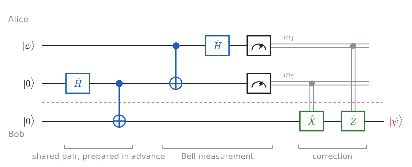
Teleportation does not clone (Alice's state is consumed by measurement), does not signal superluminally (Bob has $\frac{1}{2} \hat{I}$ until classical bits arrive), and does not transport matter.

Remark 12.12.1The two protocols are one trick

Superdense coding: one pair $+$ one qubit $\to$ two bits. Teleportation: one pair $+$ two bits $\to$ one qubit. The correction ${\hat{Z}}^{m_{1}} {\hat{X}}^{m_{2}}$ is the encoding read backwards.

12.12.4The CHSH Game

The game. A referee sends random bits $x$ to Alice and $y$ to Bob, who cannot communicate. They answer $a$ and $b$ , and win if

\begin{matrix} a \oplus b = x \land y . \end{matrix}

Theorem 12.12.4Classical bound

Any strategy fixed in advance, shared randomness included, wins at most $3$ times in $4$ .

Shared randomness averages deterministic strategies, so it suffices to rule those out. Winning all four needs

f (0) \oplus g (0) = 0, f (0) \oplus g (1) = 0, f (1) \oplus g (0) = 0, f (1) \oplus g (1) = 1 .

Adding all four modulo $2$ : each of $f (0), f (1), g (0), g (1)$ appears twice so the left is $0$ , while the right is $1$ . Three of four is achievable by always answering $0$ .

The quantum strategy. Share $| Φ^{+} ⟩$ and measure

\begin{matrix} \hat{A} (ϑ) = \cos ϑ \hat{Z} + \sin ϑ \hat{X}, \end{matrix}

Alice at $0$ or $π / 2$ , Bob at $\pm π / 4$ . On $| Φ^{+} ⟩$ , $⟨ \hat{Z} \otimes \hat{Z} ⟩ = ⟨ \hat{X} \otimes \hat{X} ⟩ = + 1$ and the cross terms vanish, so

\begin{matrix} ⟨ Φ^{+} | \hat{A} (ϑ) \otimes \hat{A} (ϑ^{'}) | Φ^{+} ⟩ = \cos (ϑ - ϑ^{'}), \Pr [agree] = \cos^{2} \frac{ϑ - ϑ^{'}}{2} . \end{matrix}

The three pairs needing agreement have differences $\mp π / 4$ , $π / 4$ ; the $(1, 1)$ pair needs disagreement at $3 π / 4$ , and $1 - \cos^{2} (3 π / 8) = \cos^{2} (π / 8)$ . All four give

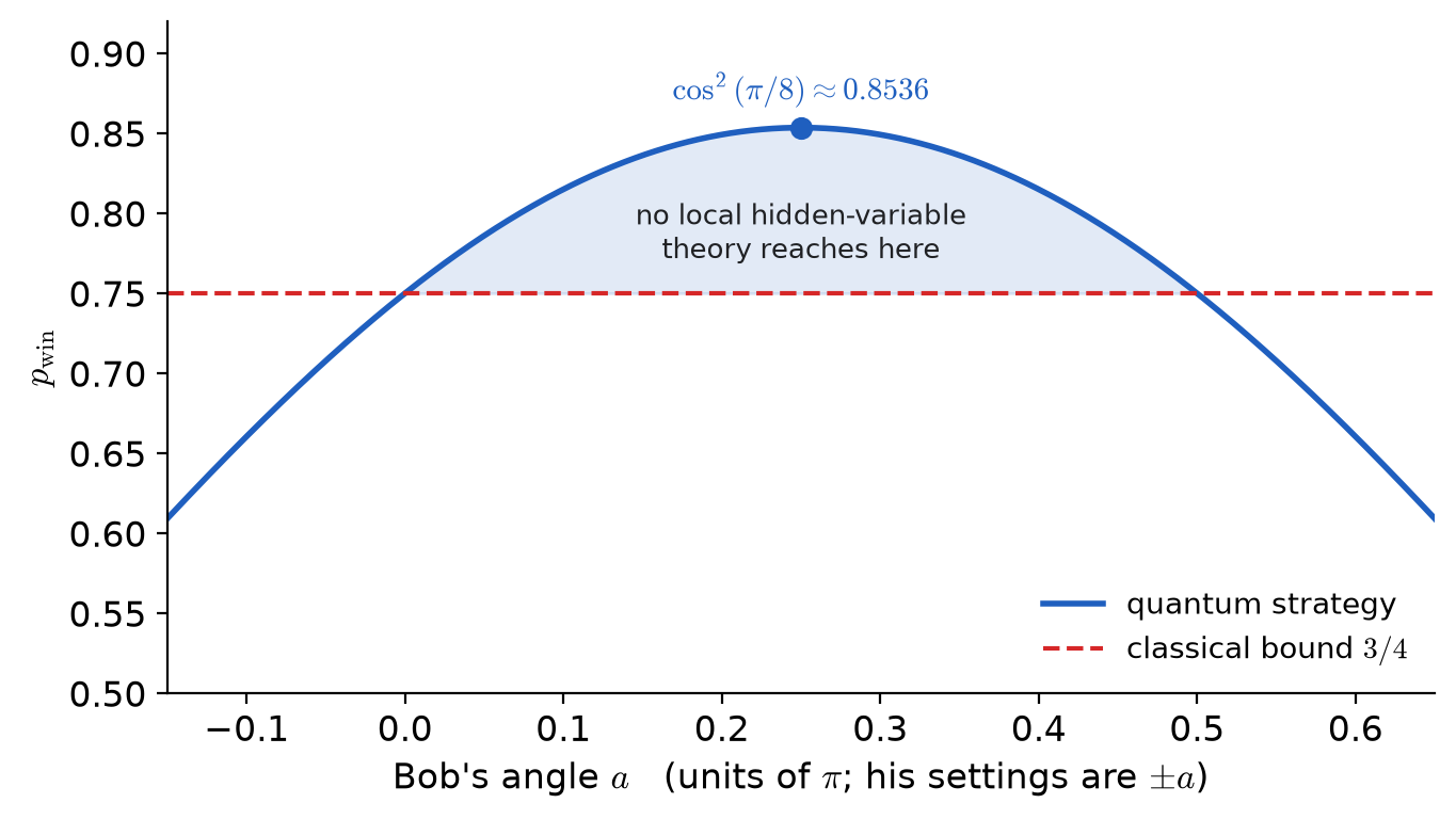
\begin{matrix} p_{win} = \cos^{2} \frac{π}{8} = \frac{2 + \sqrt{2}}{4} \approx 0.8536 \end{matrix}

Winning probability against Bob's angle, Alice's settings fixed at 0 and /2. Nothing fixed in advance rises above the dashed line, and the quantum strategy does so over a wide range — so the experiment tolerates imperfect alignment. — Figure 12.7. Winning probability against Bob's angle, Alice's settings fixed at $0$ and $π / 2$ . Nothing fixed in advance rises above the dashed line, and the quantum strategy does so over a wide range — so the experiment tolerates imperfect alignment.

As an inequality, with

\begin{matrix} S = ⟨ {\hat{A}}_{0} {\hat{B}}_{0} ⟩ + ⟨ {\hat{A}}_{0} {\hat{B}}_{1} ⟩ + ⟨ {\hat{A}}_{1} {\hat{B}}_{0} ⟩ - ⟨ {\hat{A}}_{1} {\hat{B}}_{1} ⟩, p_{win} = \frac{1}{2} + \frac{S}{8}, \end{matrix}

\begin{matrix} | S | \leq 2 (local hidden variables), | S | \leq 2 \sqrt{2} (Tsirelson) . \end{matrix}

Remark 12.12.2What the experiment settles

The failed assumption is the one used in Theorem 12.12.4: that $a$ depends only on $x$ and information carried beforehand, and $b$ only on $y$ and the same. Any such local hidden-variable theory obeys $| S | \leq 2$ . Aspect measured $S > 2$ in the early 1980s; by 2015 three groups had closed the locality and detection loopholes together; the 2022 Nobel Prize followed. Note what survives: Theorem 12.12.3 is exact. What dies is that outcomes were determined before measurement.

12.13The Density Operator

A state vector cannot represent either classical uncertainty (“ $| 0 ⟩$ or $| 1 ⟩$ , unknown to us”) or a subsystem of an entangled pair. The density operator handles both situations in one framework.

Definition 12.13.1Density operator

A system prepared in $| ψ_{i} ⟩$ with probability $p_{i}$ is

\begin{matrix} \hat{ρ} = \sum_{i} p_{i} | ψ_{i} ⟩ ⟨ ψ_{i} |, p_{i} \geq 0, \sum_{i} p_{i} = 1, \end{matrix}

pure if some $p_{i} = 1$ and mixed otherwise.

Every $\hat{ρ}$ is Hermitian, positive semidefinite, with $Tr \hat{ρ} = 1$ ; and every such operator is a state. The rules become

\begin{matrix} p_{k} = Tr ({\hat{Π}}_{k} \hat{ρ}), ⟨ \hat{A} ⟩ = Tr (\hat{A} \hat{ρ}), \hat{ρ} ⟼ \hat{U} \hat{ρ} {\hat{U}}^{†} . \end{matrix}

Example 12.13.1The two ways of being fifty-fifty

Compare $| + ⟩$ with the mixture “ $| 0 ⟩$ or $| 1 ⟩$ , each $\frac{1}{2}$ ”.

Solution.

{\hat{ρ}}_{+} = \frac{1}{2} (\begin{matrix} 1 & 1 \\ 1 & 1 \end{matrix}), {\hat{ρ}}_{mix} = \frac{1}{2} (\begin{matrix} 1 & 0 \\ 0 & 1 \end{matrix}) .

Identical diagonals: no computational-basis measurement tells them apart. The difference is entirely the off-diagonal coherences.

In the $| \pm ⟩$ basis they separate: $Tr (| + ⟩ ⟨ + | {\hat{ρ}}_{+}) = 1$ against $\frac{1}{2}$ for the mixture. The superposition is definite but looks random in one basis; the mixture is ignorance and looks random in every basis.

That is decoherence in advance: dephasing is the coherences decaying to zero, turning the first matrix into the second. No energy lost, no population moved — only the interference.

The Bloch ball. Any qubit state is

\begin{matrix} \hat{ρ} = \frac{\hat{I} + \vec{r} \cdot \vec{σ}}{2}, | \vec{r} | \leq 1, Tr ({\hat{ρ}}^{2}) = \frac{1 + | \vec{r} |^{2}}{2} . \end{matrix}

Pure states are the surface, mixed states the interior, $\frac{1}{2} \hat{I}$ the center. Now $T_{1}$ and $T_{2}$ are exact: $T_{1}$ moves $r_{z}$ , $T_{2}$ shrinks $r_{x}$ and $r_{y}$ . Dephasing is the Bloch vector collapsing onto the $z$ axis.

Reduced states. Tracing out the subsystem that is not observed,

\begin{matrix} {Tr}_{B} (| a b ⟩ ⟨ a^{'} b^{'} |) = ⟨ b^{'} | b ⟩ | a ⟩ ⟨ a^{'} |, \end{matrix}

and applying it to $| Φ^{+} ⟩$ the cross terms die because $⟨ 1 | 0 ⟩ = 0$ :

\begin{matrix} {\hat{ρ}}_{A} = {Tr}_{B} | Φ^{+} ⟩ ⟨ Φ^{+} | = \frac{1}{2} \hat{I} \end{matrix}

Alice's half is maximally mixed — a fair coin in every basis — while the joint state is pure. All the information is in the correlation and none in either part. That is why entanglement is a resource, and it completes Example 12.9.2.

12.13.1No Signalling, Proved

For a unitary on Alice's side, by cyclicity of the partial trace,

{Tr}_{A} [({\hat{U}}_{A} \otimes \hat{I}) \hat{ρ} ({\hat{U}}_{A}^{†} \otimes \hat{I})] = {Tr}_{A} [({\hat{U}}_{A}^{†} {\hat{U}}_{A} \otimes \hat{I}) \hat{ρ}] = {\hat{ρ}}_{B} .

For an unreported measurement the state is $\sum_{k} ({\hat{Π}}_{k} \otimes \hat{I}) \hat{ρ} ({\hat{Π}}_{k} \otimes \hat{I})$ , and the same step with $\sum_{k} {\hat{Π}}_{k} = \hat{I}$ again gives ${\hat{ρ}}_{B}$ .

12.14Obstacles

Decoherence. The qubit entangles with uncontrolled environmental degrees of freedom. Tracing out the environment drives ${\hat{ρ}}_{+} \to {\hat{ρ}}_{mix}$ by suppressing coherences.

Gate errors compound. With error $ϵ$ per gate a circuit of $N$ gates is about $(1 - ϵ)^{N}$ likely to be right, so $10^{- 3}$ allows a few hundred gates.

Error correction. No-cloning forbids copy-and-vote. Instead one logical qubit is spread over many physical ones and only parity relations are measured — revealing that an error occurred without revealing the state. Current estimates: $10^{2}$ to $10^{3}$ physical qubits per logical one.

Scale. Shor's algorithm on a cryptographic number is usually estimated at millions of physical qubits; present machines have hundreds to low thousands, each needing control and readout wiring at $10$ mK.

The core physics is established; the main challenge is engineering scale and fault tolerance. The algorithms are mathematically sound and the foundational effects are experimentally verified. What remains is building systems large and coherent enough for practical workloads.

12.15Summary

Classical: probability vectors, stochastic matrices (Thm. 12.2.1). Quantum: amplitude vectors, unitaries (Thm. 12.5.1).
The difference is cancellation: ${\hat{H}}^{2} = \hat{I}$ while $M^{2} = M$ (Ex. 12.4.1).
Global phase is invisible, leaving the Bloch sphere, Eq. (12.8). Every single-qubit gate is a rotation of it (Thms. 12.6.1, 12.6.2).
A gate is a pulse: in the rotating frame the Hamiltonian is constant, Eq. (12.19), and the rotation angle is the pulse area.
$T_{1}$ is energy leaving, $T_{2}$ is phase becoming unknown, and $T_{2}$ is what limits computation. Figure of merit $T_{2} / t_{gate}$ . Every platform is a driven two-level system.
Two qubits: tensor product, entanglement (Def. 12.9.1), controlled gates as projector sums (Eq. (12.26)). $n$ qubits: $2^{n}$ amplitudes, and ${\hat{H}}^{\otimes n}$ makes an equal superposition with $n$ gates.
Three algorithms, all from phase kickback (Thm. 12.11.1): Deutsch learns a global property in one query, Bernstein–Vazirani extracts $n$ hidden bits in one, Grover searches in $\sqrt{N}$ — with certainty after one round when $N = 4$ .
Three impossibilities: no cloning, no perfect discrimination, no signalling. The third makes the first two consistent with entanglement.
The density operator is the general formulation. Mixture and superposition differ only in the coherences (Ex. 12.13.1); decoherence is those decaying; half a Bell pair is $\frac{1}{2} \hat{I}$ .
CHSH: at most $3 / 4$ classically, $\cos^{2} (π / 8) \approx 0.8536$ with entanglement. Measured.

12.16Exercises

Classical first. (a) Write the four functions from one bit to one bit as matrices; which are stochastic? (b) Show $M A M = M$ for every stochastic $A$ . (c) Which property of $\hat{Z}$ has no stochastic counterpart, and why does that make Example 12.4.1 possible?
Points on the sphere. For $| ψ_{1} ⟩ = \frac{1}{\sqrt{2}} (| 0 ⟩ - i | 1 ⟩)$ , $| ψ_{2} ⟩ = \frac{1}{2} | 0 ⟩ + \frac{\sqrt{3}}{2} | 1 ⟩$ and $| ψ_{3} ⟩ = \frac{i}{\sqrt{2}} (| 0 ⟩ + | 1 ⟩)$ , find $(θ, φ)$ and $\vec{r}$ . Two appear in the table of Sec. 12.5.1 — one as written, one only after a global phase is stripped. Which, and by which theorem?
Gate algebra. (a) Verify Eq. (12.13). (b) Show $\hat{X}, \hat{Y}, \hat{Z}$ pairwise anticommute and $\hat{X} \hat{Y} = i \hat{Z}$ . (c) Compute ${\hat{R}}_{{\vec{e}}_{z}}^{†} (θ) \hat{X} {\hat{R}}_{{\vec{e}}_{z}} (θ)$ and show it is $\cos θ \hat{X} - \sin θ \hat{Y}$ .
Calibration. A qubit is driven at $Ω / 2 π = 32$ MHz. (a) Find $t_{π}$ and the $π / 2$ pulse time. (b) The amplitude is $2 %$ low; find the error and compare with $1 %$ — by what factor, and why? (c) Instead detune by $1$ MHz at correct amplitude. Use Eq. (6.16) to find the maximum transfer, and show no pulse duration repairs a detuning error.
Coherence budgets. A transmon has $T_{2} = 150 μ$ s with $25$ ns gates; an ion has $T_{2} = 10$ s with $50 μ$ s gates. (a) How many gates fit in each? (b) Which finishes a $1000$ -gate circuit sooner in wall-clock time? (c) Why do the two measures disagree, and which decides whether an algorithm runs at all?
Product or entangled? Classify $\frac{1}{2} (| 00 ⟩ + | 01 ⟩ + | 10 ⟩ + | 11 ⟩)$ , $\frac{1}{\sqrt{2}} (| 00 ⟩ + | 01 ⟩)$ , $\frac{1}{\sqrt{2}} (| 00 ⟩ - | 11 ⟩)$ , $\frac{1}{\sqrt{3}} (| 00 ⟩ + | 01 ⟩ + | 10 ⟩)$ , exhibiting the factorization or the contradiction.
Circuit identities. (a) Verify Example 12.10.1 by $4 \times 4$ multiplication. (b) Show three alternating CNOTs make SWAP. (c) Show $CNOT = (\hat{I} \otimes \hat{H}) CZ (\hat{I} \otimes \hat{H})$ .
The algorithms by hand. (a) Run Deutsch for $f (x) = x$ and for $f (x) = 1$ . (b) Run Bernstein–Vazirani for $n = 3$ , $a = 101$ . (c) For Grover with $N = 8$ , compute the success probability after $1$ , $2$ and $3$ rounds and say which $k$ you would choose.
Mixtures and superpositions. (a) Write $\hat{ρ}$ for $| + i ⟩$ and for the mixture “ $| + ⟩$ or $| - ⟩$ , each $\frac{1}{2}$ ”. Which is pure? (b) Compute $Tr ({\hat{ρ}}^{2})$ for both and check Eq. (12.47). (c) Give a basis that tells them apart and one that does not.
How entangled? For $| Ψ (λ) ⟩ = \cos λ | 00 ⟩ + \sin λ | 11 ⟩$ , compute ${\hat{ρ}}_{A}$ and its Bloch vector; evaluate at $λ = 0$ and $π / 4$ ; compute $Tr ({\hat{ρ}}_{A}^{2})$ and explain why it measures entanglement.
Teleportation in full. (a) Derive Eq. (12.38). (b) If Bob measures immediately, show his statistics are $50 / 50$ regardless of $α, β$ . (c) If he applies $\hat{X}$ instead of $\hat{I}$ , what is $| ⟨ ψ | ψ^{'} ⟩ |^{2}$ ?
CHSH both ways. (a) List the $16$ deterministic strategies and confirm the maximum is $3$ . (b) Compute $S$ for the angles of Sec. 12.12.4. (c) Bob mis-aligns by $10^{\circ}$ ; recompute $p_{win}$ and say whether $3 / 4$ is still beaten.

12.17Project: Two Qubits, From Scratch

The problem. Write a two-qubit simulator in about fifty lines of numpy and use it to reproduce every quantitative claim in this chapter.

No quantum library needed: a state is a length-four complex array, a gate a $4 \times 4$ matrix, and numpy.kron builds both. Writing it yourself is the point — the conventions of Remark 12.9.1 only become real when you must choose one.

On paper. Work out by hand the matrices of $\hat{H} \otimes \hat{I}$ , $\hat{I} \otimes \hat{H}$ and $CNOT$ in the ordering of Eq. (12.23). A simulator debugged against its own output is not debugged.
On the computer. Build it: single-qubit gates, a function lifting one to a chosen wire, $CNOT$ from Eq. (12.26) as a sum of Kronecker products (not typed in by hand), and a measurement routine. Check every gate is unitary to machine precision.
On the computer. Prepare all four Bell states; compute ${\hat{ρ}}_{A}$ by partial trace and confirm Eq. (12.49). Then teleport a random $| ψ ⟩$ branch by branch and confirm fidelity $1$ on all four.
On the computer. Implement Grover for $N = 4$ and confirm Example 12.11.2 — probability $1$ after one round. Then do $N = 8$ and plot success against rounds, reproducing Fig. 12.5. Note where it peaks and falls.
On the computer. Play CHSH: implement Eq. (12.40) as a measurement in the rotated basis, sample $10^{5}$ rounds, and report the winning fraction with its statistical error. It should sit at $0.8536$ .
On the computer. Add dephasing: apply $\hat{Z}$ to one qubit with probability $p$ , averaging the two cases — which is Example 12.13.1, so use density operators. Plot $p_{win}$ against $p$ and find where the advantage disappears.
What has to move. One animation: a Bloch sphere tracing a resonant $π$ pulse, beside the same pulse detuned by $Ω / 2$ so the vector precesses about a tilted axis and misses the south pole. Caption it with the fact that driving longer cannot fix the miss.

The check. Part (c) is the real test: teleportation must succeed on all four branches. One branch failing means a sign error in the correction table, two means inconsistent qubit ordering, four means the partial trace is wrong.

Be ready to answer. Part (e) beat the classical bound, yet your simulator is a deterministic classical program. Explain why that is not a contradiction, and name the assumption of Theorem 12.12.4 your program violates.

For the Interested Reader

Videos

Video

The Map of Quantum Computing - Quantum Computing Explained

Watch on YouTube

Open video on YouTube

The companion to Remark 12.1.1: the whole field on one page, walked through in half an hour. The hardware of Sec. 12.8.1 and the obstacles of Sec. 12.14 are all on it.

Websites

https://quantum.cloud.ibm.com/learning/en/courses/basics-of-quantum-information IBM Quantum Learning, Basics of Quantum Information — the four-lesson course this chapter condenses, with runnable Qiskit code for Secs. 12.9–12.12.
IBM Quantum Learning — the rest of their courses, including the algorithms of Sec. 12.11 in more depth.
Google Quantum AI — their research programme, hardware and error-correction results.
Cirq — Google's circuit framework; a useful second opinion on the conventions of Remark 12.9.1.
https://www.quantum-inspire.com/kbase/introduction-to-quantum-computing/ Quantum Inspire knowledge base — short articles on the hardware, from a group that builds it.

12.1Introduction

12.2Classical Information

12.3Quantum Information

12.3.1Measurement

12.3.2Global Phase

12.4What Makes Quantum Information Useful

12.5Qubits and Gates

12.5.1The Bloch Sphere

12.5.2What a Gate Is

12.6Single-Qubit Gates

12.6.1Every Gate Is a Rotation

12.7Making a Gate: From Pulse to Rotation

12.8Coherence and Hardware

12.8.1What Qubits Are Made Of

12.9Two Qubits

12.9.1Entanglement

12.9.2Controlled Gates

12.10Many Qubits

12.10.1Universality

12.11Three Quantum Algorithms

12.11.1The Oracle and Phase Kickback

12.11.2Deutsch: One Query Instead of Two

12.11.3Bernstein–Vazirani: n Bits in One Query

12.11.4Grover: Searching in N

12.12What Entanglement Is Good For

12.12.1Three Impossibilities

12.12.2Superdense Coding

12.12.3Teleportation

12.12.4The CHSH Game

12.13The Density Operator

12.13.1No Signalling, Proved

12.14Obstacles

12.15Summary

12.16Exercises

12.17Project: Two Qubits, From Scratch

For the Interested Reader

Videos

Websites

12.11.3Bernstein–Vazirani: $n$ Bits in One Query

12.11.4Grover: Searching in $\sqrt{N}$